
Wavelet-based Circular Hough Transform
and Its Application in Embryo Development Analysis
Marcelo Cicconet
1
, Davi Geiger
2
and Kris Gunsalus
1
1
Center for Genomics and Systems Biology, New York University, New York, U.S.A.
2
Courant Institute of Mathematical Sciences, New York University, New York, U.S.A.
Keywords:
Machine Vision, Circular Hough Transform, Biological Cells.
Abstract:
Detecting object shapes from images remains a challenging problem in computer vision, especially in cases
where some a priori knowledge of the shape of the objects of interest exists (such as circle-like shapes) and/or
multiple object shapes overlap. This problem is important in the field of biology, particularly in the area
of early-embryo development, where the dynamics is given by a set of cells (nearly-circular shapes) that
overlap and eventually divide. We propose an approach to this problem that relies mainly on a variation of
the circular Hough Transform where votes are weighted by wavelet kernels, and a fine-tuning stage based
on dynamic programming. The wavelet-based circular Hough transform can be seen as a geometric-driven
pulling mechanism in a set of convolved images, thus having important connections with well-stablished
machine learning methods such as convolution networks.
1 INTRODUCTION
Information about cell division timing and cell shape
are some of the features used to analyze the early
stages of life in research and medicine. These fea-
tures are used to study the roles of different genes in
early development and to evaluate the quality of in
vitro fertilized (IVF) embryos in fertility clinics. As
data from automated time-lapse imaging of embryos
accumulates, data analysis becomes the bottleneck of
the research process Therefore, being able to count
cells and analyze their shape automatically is critical.
One may see the problem simply as that of de-
scribing shapes from a given set of points. This is
the approach of the Hough Transform (HT) (Duda
and Hart, 1972). However, the original implementa-
tion, where votes are considered pixel-wise, is very
sensitive to noise. Recent works approach the is-
sue by weighting votes with kernels (Fernandes and
Oliveira, 2008; White et al., 2010). Our method goes
in a similar direction extending it to overlapping ob-
jects and cell division. Furthermore, we propose that,
by interpreting the HT as a geometric mechanism for
pulling information from a set of convolutions, impor-
tant connections with recent developments in machine
learning algorithms can be established.
In this realm, one intuitive and recently developed
learning technique is “Deep Learning with Convolu-
tion Networks” (Hinton, 2007; LeCun et al., 2010).
Great progress was made just recently on understand-
ing this problem further with the work of Bruna and
Mallat (2012). They argue that each layer of the con-
volution network, where a convolution is applied fol-
lowed by a pooling mechanism, is equivalent to a
wavelet transform followed by the measurement of
an invariant (the magnitude of the transform). They
interpret the succession of convolution networks in
deep learning as to describe the data as a concatena-
tion of invariant descriptions of it. However, at least
one question remains: what is the “meaning” of the
last step of the convolution networks where a linear
classifier is applied to the output of the last layer of
the convolution network (instead of a pooling)?
We see these issues as a source of inspiration
to propose a bottom-up model for shape detection
starting with wavelet filtering, followed by a HT for
known shapes, and a dynamic programming tech-
nique to fine-tune the HT results.
We apply our method to mouse-embryo cell track-
ing and division detection up to the 4-cell stage. Our
work is being used at the NYU Center for Genomics
and Systems Biology to analyze the influence of par-
ticular genes in the timing dynamics of the first cells.
Our method performs almost twice as well as previ-
ously reported results on a similar problem (see Sub-
section 3.2).
669
Cicconet M., Geiger D. and Gunsalus K..
Wavelet-based Circular Hough Transform and Its Application in Embryo Development Analysis.
DOI: 10.5220/0004296006690674
In Proceedings of the International Conference on Computer Vision Theory and Applications (VISAPP-2013), pages 669-674
ISBN: 978-989-8565-47-1
Copyright
c
2013 SCITEPRESS (Science and Technology Publications, Lda.)

2 WAVELET-BASED CIRCULAR
HOUGH TRANSFORM
In the original HT, given a radius r, each edge pixel
p in the image votes for all possible centers of circles
(usually within the boundaries of the image) of radius
r passing through it.
In our implementation, given p and r, we compute
votes in a rather small “electorate”: n pixels (usually
n = 16) at equally spaced locations along the bound-
ary of the circle centered in p with radius r. The
votes of the chosen pixels are actually a weighted sum
of their neighbors’ votes, the weights being given by
a properly rotated Morlet filter, as illustrated in Fig-
ure 1.
Figure 1: The likelihood that there is a circle of radius r
centered at point p depends on the votes of n (in this case
n = 16) equally spaced points along a circle of radius r cen-
tered at p. Each voting point represents its neighbors ac-
cording to a Morlet-wavelet kernel whose orientation de-
pends on its angle. The scale is chosen beforehand, based
on the size of the image.
Implementation-wise, it is better to use convolu-
tion functions and compute the votes for a particular
angle in the circle separately, adding them in the end.
If, for instance, we look for votes in 16 equally spaced
points along a circle, then 16 convolutions need to be
performed. The sub-image where each convolution
is applied depends on the angle of the point. Fig-
ure 2 shows the implementation of such convolutions
in Matlab. The function computes the accumulator
image (L), and the (inverse) likelihood (l) that an im-
age contains a circle of a particular radius.
If an image is known to have a circle of radius r,
the point where L has its maximum is the center of
that circle. The output l indicates how spread out are
the weights in L. The idea is that if there is a well-
defined circle in the image, than a well-defined peak
will appear in L, and the value of l will be smaller
Figure 2: Matlab implementation of the accumulator image
(L) and inverse circle likelihood (l) for the Morlet-kernel
based circular HT. G: euclidian norm of gradient of the im-
age; rad: radius; nor: number of orientations (angles) con-
sidered; morlet(): function that computes the real and
imaginary parts of a Morlet-wavelet kernel (we are using
only the real part).
than if there were no circle of that radius in the image
(see Figure 3).
Circle likelihood measures the inverse likelihood
that an image contains a circle of a particular radius.
Let A be the accumulator image obtained by the cir-
cular HT algorithm
1
. We define the (inverse) circle
likelihood l as
l =
1
mn
m
∑
i=1
n
∑
j=1
A(i, j) ,
where m and n are the height and width of A, respec-
tively. This is of course simply the mean of the ele-
ments in A. To see why l reflects the inverse likeli-
hood that there is a circle of radius r in the image, let
us suppose that the accumulator A of the circular HT
was computed for radius r. We notice, first, that A is
normalized (its maximum is 1). Now, let us sort the
elements of A according to their magnitude, obtaining
a vector that we call a, with m·n entries, ranging from
close to 0 (on the left) to 1 (on the right). The value
of
1
mn
∑
mn
i=1
a(i) (that is, l) is superiorly limited by 1.
If there is a circle of radius r in the image, the curve
{i,a(i)} will have a sharper peak on the far right (that
1
The relationship between A and L is made clear in the
algorithm shown in Figure 3.
VISAPP2013-InternationalConferenceonComputerVisionTheoryandApplications
670
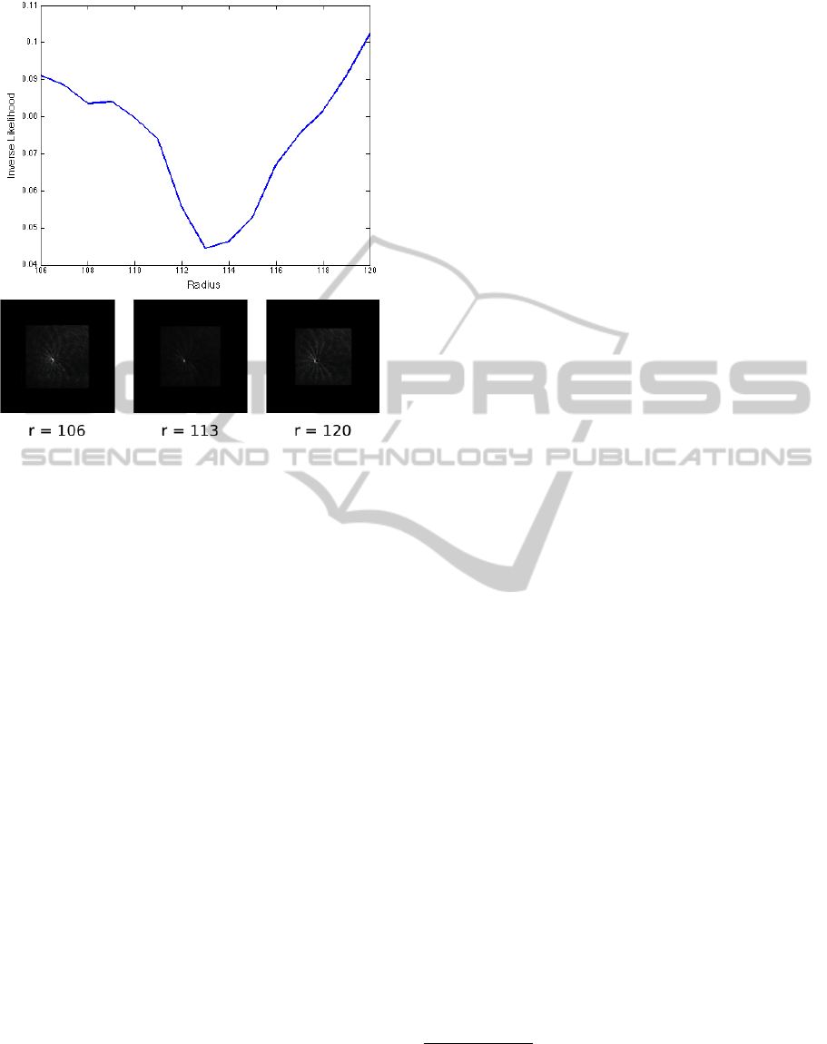
Figure 3: We introduce a measure of the likelihood that an
image contains a circle of a particular radius. The likelihood
is based on the accumulator image of a circular HT com-
puted using Morlet-wavelet filters. The top figure shows
how the inverse of the measure varies for different radii.
The figures at the bottom show the accumulator of the HTs
for the shows radii (normalized and squared, to highlight
the peaks).
is, l will be smaller) than it would otherwise. The fact
that l is superiorly limited by 1 is important because
the size of A varies for different radii (see implemen-
tation in Figure 2).
Computing the accumulator image A can be seen
as a pulling mechanism. For each candidate to be the
center of a circle one is looking for, a number of filter
outputs are “pulled” from a bank of convolved im-
ages. The choice of convolved images and areas in
these images is stablished by the prior knowledge of
what geometrical shape one is trying to find (in our
specific case, a circle of a particular radius).
3 APPLICATION
Morphological and kinetic features have been in-
creasingly used in in vitro fertilization clinics to im-
prove embryo quality assessment (Meseguer et al.,
2011). Those features include cleavage (division)
times, blastomere size, multi nucleation, cleavage du-
ration, lack of division in one or more cells, and cell-
boundary texture, to cite a few. Besides viability for
re-implantation, these features are also useful, in the
case of model systems like mouse-embryos, in the
study of the function of particular genes in embryonic
development.
Modern incubators are equipped with built-in
cameras designed to acquire time-lapse images of em-
bryos (at intervals of a few minutes). In general, these
videos are used by embryologists and researchers for
visual inspection, but research aiming at automati-
cally analyze them is emerging.
Two recent works (Meseguer et al., 2011; Wong
et al., 2010) focus on the correlation between re-
implantation viability and the interval between divi-
sion onsets (up to the 4- or 5-cell stage). In order to
obtain such information automatically, tracking of in-
dividual cells and detection of cell divisions are nec-
essary
2
.
In this section we show how the algorithm intro-
duced previously can be helpful in the problem of
tracking the cells and detecting cell division in the
early phases of mouse-embryo development (up to the
4-cell stage).
3.1 Cell Tracking and Division
Detection
Our method applies to a sequence of frames contain-
ing one (centralized) embryo only. The initial radius
is fixed (to be 110 pixels), as the size of the first cell
is roughly constant across embryos.
After pre-processing (adaptive histogram equal-
ization), the gradient (euclidian) norm of the image
is computed, and the result divided by its maximum,
providing an image in the range [0,1]. From this re-
sulting gradient image, a band around the initial cir-
cle is extracted. More specifically, n
1
equally spaced
points along the circle are sampled, and for each of
these points, n
2
points are sampled along the line per-
pendicular to the circle at that point, and centered at
that point. n
1
and n
2
vary according to the generation
of the cell. For the first cell their values are n
1
= 160
and n
2
= 100. Figure 4 illustrates this process.
We then apply dynamic programming (as in
Geiger et al. (1995)) to fine-tune the location of the
boundary of the cell. Figure 4 (c) shows what a solu-
tion looks like.
As the variance of the curvature of the boundary of
the cell is not high, we sample 16 “reference points”
in the resulting solution (which corresponds to the
fined-tuned boundary) at equally spaced intervals, and
interpolate them using cubic splines. Examples of the
2
For some works that approach the problem of cell
tracking and cell-division detection in contexts other than
early embryo development, we refer the reader to Zim-
mer et al. (2002), Dzyubachyk et al. (2010), Zimmer et al.
(2002), Huh et al. (2011), and Hamahashi et al. (2007).
Wavelet-basedCircularHoughTransformandItsApplicationinEmbryoDevelopmentAnalysis
671
(a)
(b)
(c)
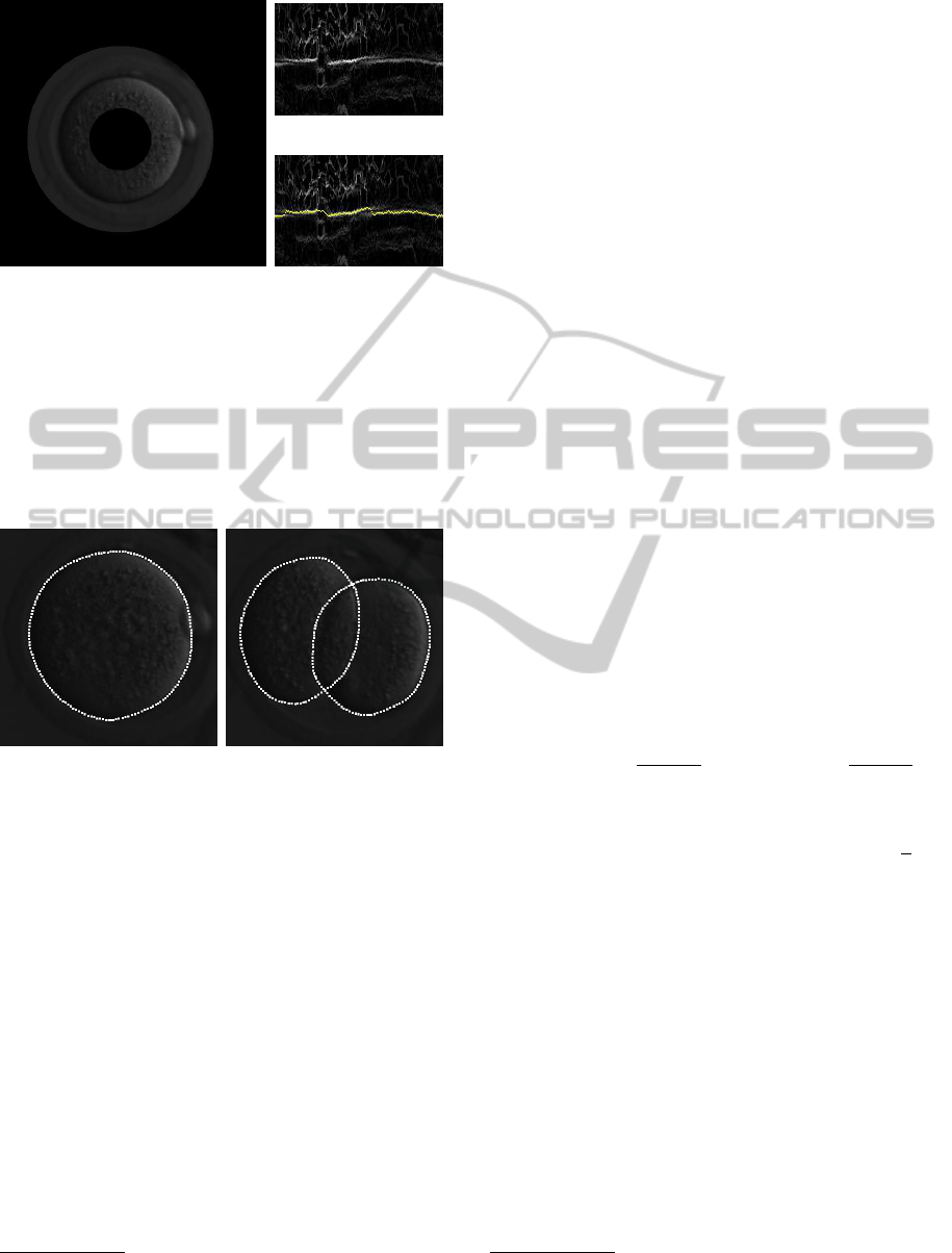
Figure 4: For each frame, there is an initial guess for the
circle that better approximate the boundary of each cell.
Following this circle around, a band of the original image
is taken (a) and mapped to a rectangular image. In fact,
the band of the original image is shown here just for il-
lustrative purposes. The computation of the boundary is
actually made using the band around the gradient of the
adaptive-histogram-equalized image (b). The yellow line
in (c) shows the solution by dynamic programming that fits
the boundary.
Figure 5: Output of the cell-boundary fitting method based
on dynamic programming.
final result for cell boundary fitting are shown in Fig-
ure 5.
The initial guess for the boundary of the cell in the
next frame is set as the circle whose center and radius
are estimated
3
according to the curve that best fit the
boundary of the cell in the previous frame. The reason
a circle is passed to the next frame, and not the actual
boundary, is that, first, cell boundaries are roughly cir-
cular; second, the dynamic programming step recov-
ers the minor differences in the next frame’s bound-
ary; and, third, the circle poses a global restriction for
the overall shape of the boundary, without which there
would be no safeguards for a non-plausible boundary
line (like one with self intersections). n
1
and n
2
are
computed according to the estimated radius for the
cell.
3
The center is the mean and the radius is the average
distance to the mean.
function rd = radiusforgeneration(g,r1)
rd = r1;
if g > 1
for i = 1:g-1
v = 4/3*pi*rdˆ3;
v = v/2;
rd = power(v/4*3/pi,1/3);
end
end
end
In the above listing, g is the generation of the cell
(1, 2, ...), and r1 is the estimated radius for a 1st gen-
eration cell. The function radiusforgeneration as-
sumes that, when a cell divides, the total volume is
kept constant
4
. n
1
is set to the integer closer to 1/4 of
the length of a circle of radius rd, and n
2
is set to the
integer closer to rd.
For a cell that is dividing, the current boundary
approximation should be replaced by two new bound-
aries. At this point, the accumulator image of the
wavelet-based circular HT for radius equal to the esti-
mated radius of the daughter cells is used to obtain the
first approximation for the centers of the new cells.
Let c be the center of the cell which is dividing,
and p the farthest point in its boundary. The centers
of the new cells are estimated to be close to the line
cp (as the dividing cell is elongated in this direction).
More precisely, let d = kp −ck, and r the estimated
radius of the daughter cells. Let c
0
and c
1
be the esti-
mated centers of the daughter cells. We set
c
0
= c + (d −r)
p −c
kp −ck
, c
1
= c −(d −r)
p −c
kp −ck
.
The final estimations for the centers of the new cells
are obtained by finding the maxima of the accumu-
lator function at the squares of edges kc
1
−c
0
k
√
2/2
centered at c
0
and c
1
. Figure 6 illustrates this.
We use three “experts” to decide when a cell is
dividing: pixel variances in the whole image, pixel
variances in the band around the boundary of a cell,
and the (inverse) circle likelihood (introduced in the
previous section).
Pixel variance is simply the variance of the pixel
value along a window of frames. We use a 5-frame
window in our implementation. Both the sum of the
pixel variances for the whole image and for a band
around each of the cell boundaries are observed. Fig-
ure 7 shows these two measures for some frames
around the frame where the first cell undergoes di-
vision.
Now, if, for instance, the estimated radius for a
4
This hypothesis is verified to be true when the esti-
mated cell volumes are computed after tracking.
VISAPP2013-InternationalConferenceonComputerVisionTheoryandApplications
672
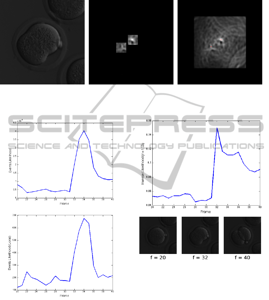
Figure 6: During division (left), the accumulator image of the circular HT with radius equal to the estimated radius of the
daughter cells is used to detect the centers of the two new cells. Regions where the new centers should be found (middle)
are estimated based on the current boundary, and the maxima of the accumulator image in these areas provide a better
approximation for the centers (right).
Figure 7: The sum of the pixel-variances in a window of 5
frames (top figure) is used (in combination with other mea-
surements) to detect a cell is dividing. The bottom figure
shows such variance computed only on a band around the
boundary of the cell. The cell divides in frame 32.
cell is r and we compute l for the circular HT cor-
responding to r in a sequence of frames, when the
cell eventually divides the value of l will increase (for
there is less evidence for a circle of radius r in the
Figure 8: The top figure shows how the inverse likelihood of
a circle of radius 113 (pixels) varies in a sequence of frames
where a cell (whose radius is approximately 113) divides.
Notice how it increases when the cell undergoes division
(frame 32). The bottom shows frames before, during, and
after cell division.
analyzed image). Figure 8 illustrates this.
Let us call v(t) and v
c
(t) the sum of pixel vari-
ances in the whole frame t and in the band around the
boundary of cell c in frame t, respectively. Also, let us
define l
g
(t) as the (inverse) likelihood curve at frame
t for a circle or radius corresponding to a cell of gen-
eration g.
The first division is detected by looking for a
sharp increase in v(t) ·v
c
(t) ·l
1
(t). Similarly, the sec-
Wavelet-basedCircularHoughTransformandItsApplicationinEmbryoDevelopmentAnalysis
673

ond division is detected by observing a variation in
v(t) ·(v
c
1
(t) + v
c
2
(t)) ·l
2
(t). (At this point, c
1
and c
2
are the two current second-generation cells.) To know
which of the cells divided, v
c
1
(t) and v
c
2
(t) are com-
pared. The third division is detected by observing
v(t) ·v
c
j
(t) ·l
2
(t), where c
j
is the second-generation
cell that remained to divide.
3.2 Results
Our cell-tracking and division-detection method suc-
cessfully applies to a total of 63 embryos. Of these, 24
were used for parameter fitting. That is, after the core
of the algorithm was implemented, we deployed it on
24 “training” cases, manually tuning the parameters
related with division detection in order to fit the data.
After this phase, the algorithm was applied to a “test”
set comprising 150 embryos. In this set, the method
correctly performed up to the first cell division in 91
cases (61%), up to the second cell division in 50 cases
(33%), and up to the third cell division (4-cell stage)
in 39 cases (26%).
In comparison to other works, the only method we
know of approaching a similar problem (Wong et al.,
2010) is reported to work (up to the 4-cell stage) for
14 embryos in a set of 100 (see p. 1117 of the men-
tioned reference). Apart from performance compar-
isons, we emphasize that features like the circle like-
lihood and the wavelet-based HT are more interesting
in theoretical terms, as they provide high level repre-
sentations of what happens in the (sequence of) im-
ages (as opposed to the “brute force” approach of a
particle filters tracker, for instance).
4 CONCLUSIONS
We introduced a circular HT implementation de-
signed as a pulling mechanism on a set of images con-
volved with Morlet-wavelets filters. As a byproduct
of the algorithm that computes the accumulator for
the circular HT of a particular radius, we compute the
(inverse) likelihood that an image contains a circle of
that radius.
Both the accumulator image and the circle like-
lihood are applied in a method for cell division on-
set detection and cell boundary tracking for the case
of mouse-embryos in the early stage of development
(from 1 to 4 cells). The method is in current use in a
biology lab, and outperforms previously reported re-
sults for a similar problem (see previous section).
REFERENCES
Bruna, J. and Mallat, S. (2012). Invariant scattering convo-
lution networks. CoRR, abs/1203.1513.
Duda, R. O. and Hart, P. E. (1972). Use of the hough trans-
formation to detect lines and curves in pictures. Com-
mun. ACM, 15(1):11–15.
Dzyubachyk, O., van Cappellen, W., Essers, J., Niessen, W.,
and Meijering, E. (2010). Advanced level-set-based cell
tracking in time-lapse fluorescence microscopy. Medical
Imaging, IEEE Transactions on, 29(3):852 –867.
Fernandes, L. A. and Oliveira, M. M. (2008). Real-time line
detection through an improved hough transform voting
scheme. Pattern Recognition, 41(1):299 – 314.
Geiger, D., Gupta, A., Costa, L., and Vlontzos, J. (1995).
Dynamic programming for detecting, tracking, and
matching deformable contours. Pattern Analysis and
Machine Intelligence, IEEE Transactions on, 17(3):294
–302.
Hamahashi, S., Kitano, H., and Onami, S. (2007). A system
for measuring cell division patterns of early caenorhab-
ditis elegans embryos by using image processing and ob-
ject tracking. Syst. Comput. Japan, 38(11):12–24.
Hinton, G. E. (2007). Learning multiple layers of represen-
tation. Trends in Cognitive Sciences, 11:428–434.
Huh, S., Ker, D., Bise, R., Chen, M., and Kanade, T. (2011).
Automated mitosis detection of stem cell populations in
phase-contrast microscopy images. Medical Imaging,
IEEE Transactions on, 30(3):586 –596.
LeCun, Y., Kavukcuoglu, K., and Farabet, C. (2010). Con-
volutional networks and applications in vision. In ISCAS
2010), May 30 - June 2, 2010, Paris, France, pages 253–
256. IEEE.
Meseguer, M., Herrero, J., Tejera, A., Hilligsoe, K., Ram-
sing, N., and Remohi, J. (2011). The use of morphoki-
netics as a predictor of embryo implantation. Human Re-
production, 26(10):2658–71.
White, A. G., Cipriani, P. G., Kao, H.-L., Lees, B., Geiger,
D., Sontag, E., Gunsalus, K. C., and Piano, F. (2010).
Rapid and accurate developmental stage recognition of
c. elegans from high-throughput image data. In CVPR,
pages 3089–3096.
Wong, C. C., Loewke, K. E., Bossert, N. L., Behr, B., Jonge,
C. J. D., Baer, T. M., and Pera, R. A. R. (2010). Non-
invasive imaging of human embryos before embryonic
genome activation predicts development to the blastocyst
stage. Nature Biotechnology, 28:1115–21.
Zimmer, C., Labruyere, E., Meas-Yedid, V., Guillen, N.,
and Olivo-Marin, J.-C. (2002). Segmentation and track-
ing of migrating cells in videomicroscopy with paramet-
ric active contours: a tool for cell-based drug testing.
Medical Imaging, IEEE Transactions on, 21(10):1212 –
1221.
VISAPP2013-InternationalConferenceonComputerVisionTheoryandApplications
674
