Analysis of MIMO Systems with Transmitter-side Antennas Correlation

Francisco Cano-Broncano

, C´esar Benavente-Peces

, Andreas Ahrens

Francisco Javier Ortega-Gonz´alez

and Jos´e Manuel Pardo-Mart´ın

Universidad Polit´ecnica de Madrid, Ctra. Valencia. km. 7, 28031 Madrid, Spain

Hochschule Wismar, University of Technology, Business and Design, Philipp-M¨uller-Straße 14, 23966 Wismar, Germany

Keywords:

Multiple Input Multiple Output, Antennas Correlation, Wireless Communication.

Abstract:

Due to its potential performance multiple input multiple output (MIMO) systems are being included in the

current standard developments. Nevertheless issues like antennas proximity at the transmitter and receiver

arrays can limit the achievable performance. Antennas proximity produces a phenomenon called correlation

which affects the channel performance by reducing the capacity and increasing the BER. Hence, the aim of

this paper is investigating the transmitter-side antennas correlation modelling and effects. Together with the

appropriate signal processing (e. g. singular values decomposition), the effect of transmitter-side antennas

correlation is studied. Our results show that under the effect of antennas correlation not necessarily all layers

might be used for the data transmission since the weighting of the stronger layer within the MIMO system

becomes even stronger respect to non-correlated channels. Simulation results are shown to underline these

effects.

1 INTRODUCTION

Multiple Input Multiple Output (MIMO) systems

have been studied during the last decades due to their

ability to increase the channel capacity and decrease

the bit error rate (BER) without increasing the trans-

mit power needed at the transmitter side. In order to

obtain the full advantages of the MIMO systems per-

fect channel state information is required at both the

transmitter and receiver sides in order to perform the

appropriate signal processing tasks at the transmit-

ter (pre-processing) as well as at the receiver (post-

processing) side. A popular technique used for those

signal processing operations is the singular values de-

composition (SVD). By introducing both operations

inter-antenna interferences are avoided and the full

MIMO system capabilities can be exploited assuming

a highly scattered environment. Due to the antennas

physical proximity compared to the wavelength addi-

tional effects must be taken into consideration in the

analysis and implementation of a MIMO system. Un-

der that condition antennas correlation effect appears

affecting the MIMO channel capacity and (bit-error

rate) BER. MIMO systems require a highly scattered

environment in order to beneﬁt from the use of multi-

ple antennas to select the appropriate transmit and re-

ceive conditions. This is synonymous of having mul-

tiple paths which largely differ.

Unfortunately, due to the proximity of the an-

tennas separation the theoretically degree of design-

freedom of the MIMO system decreases (Lee, 1973;

Ertel et al., 1998; Wang et al., 2009). In the pres-

ence of antennas correlation the environment is less

scattered and hence the MIMO channel capacity de-

creases and the BER rises. Antennas correlation im-

plies the similarity in the antennas paths and in conse-

quence the environment becomes less scattered. This

means that the off-diagonal elements of the channel

matrix become similar and it is not possible to exploit

the full capabilities of the MIMO system any longer.

In order to predict the effects of antenna correlation

a proper correlation model is required. The effect of

antennas correlation can be separated into two inde-

pendent effects: the one corresponding to transmitter-

side antennas correlation and that due to receiver-side

antennas correlation. In order to analyse and pre-

dict the behaviour of a correlated MIMO system two

key points must be solved: The ﬁrst one concerns the

model of the antennas correlation (i. e. the description

of the correlation coefﬁcients) and the second one is

related to analysing the correlation effect compared to

an uncorrelated MIMO system.

The antennas correlation is usually described by

the antennas correlation matrices one for transmitter-

side and other for receiver-side (assuming indepen-

dence between correlations) which collect the cor-

147

Cano-Broncano F., Benavente-Peces C., Ahrens A., Ortega-González F. and Pardo-Martín J..

Analysis of MIMO Systems with Transmitter-side Antennas Correlation.

DOI: 10.5220/0004228401470155

In Proceedings of the 3rd International Conference on Pervasive Embedded Computing and Communication Systems (PECCS-2013), pages 147-155

ISBN: 978-989-8565-43-3

 2013 SCITEPRESS (Science and Technology Publications, Lda.)

relation coefﬁcients between the antennas, while the

global effect is represented by a called system corre-

lation matrix which is the Kronecker product (Laub,

2005) between the transmitter and receiver side an-

tennas correlation matrices (Taparugssanagorn et al.,

2006; Salz and Winters, 1994; Shiu et al., 2000).

In (Yueyu and Lili, 2007) the antennas correlation

effect on the channel capacity is studied when using a

circular array compared to a linear one showing the

decrease in the channel capacity with the antennas

correlation effect.

This paper is aimed at the analysis of MIMO sys-

tems performance in the presence of transmitter-side

antennas correlation. The main contribution of this

paper is the deﬁnition of the correlation coefﬁcients

between transmitter-side antennas as a function of the

main parameters showing how they affects the char-

acteristic of the layer-speciﬁc weighting factors.

In this paper linear antennas arrays are studied.

The authors do not focus on concrete spatial antennas

distributions. Instead they use a general propagation

model in order to compute the correlation coefﬁcient

between antennas.

The remaining part of this contribution is orga-

nized as follows: Section 2 describes the physical an-

tennas adjustment as well as the corresponding vari-

ables that will impact the computation of the anten-

nas correlation. The corresponding correlated MIMO

system model is introduced in Section 3. The associ-

ated performance results are presented and interpreted

in section 4. Finally, in section 5 the concluding re-

marks are discussed.

2 BASE-STATION RELATED

ANTENNAS CORRELATION

This section describes the physical antennas adjust-

ment as well as the corresponding variables that will

impact the computation of the antennas correlation.

Starting with the analysis of the correlation between

any pair of transmit antennas with respect to a given

receive antenna, the result will be extended to any an-

tennas conﬁguration as the correlation is computed

for each antennas pair separately. At ﬁrst, only line of

sight (LOS) trajectories are considered as highlighted

in Fig. 1.

Fig. 1 represents the physical set-up for a pair of

transmit antennas and one receive antenna. The dis-

tance between the receive antenna and the reference

point (centre of the physical disposition) of the trans-

mit antennas is D. The distance between the transmit

antenna #1 and the receive antenna is d

, while the

distance between the transmit antenna #2 and the re-

d/2

antenna #1

antenna #2

Figure 1: Antennas’ physical disposition: two transmit and

one receive antennas.

ceive antenna is d

. The transmit antennas itself are

separated by the distance d. Considering the spac-

ings and angles introduced in Fig. 1 some relations

can be stated for each transmit antenna. Considering

transmit antenna #1, the following relation can be es-

tablished:

·cos(α

) = D−

·cos(φ) . (1)

Equation (1) describes the relation among the various

physical parameters described in Fig. 1. A similar re-

lation can be obtained for transmit antenna #2 dealing

with the following relation:

·cos(α

) = D+

·cos(φ) . (2)

Now, the focus is set on the computation of the corre-

lation between transmit antennas. Here, the antennas

set-up shown in Fig. 1 is considered. Let’s assume

that the same signal s(t) is simultaneously transmitted

through the transmit antennas #1 and #2. Under this

conditions the signals arriving at the receive antenna

can be described as follows: The signal arriving at the

receive antenna from transmit antenna #1 is given by:

(t) = s(t) ·G

·A(d

) ·e

−j2πd

/λ

, (3)

where G

describes the transmit antenna #1 radia-

tion pattern gain in the direction of departure and

A(d

) ≤ 1 describes the path attenuation effect (given

in terms of gain) for the distance d

. The complex

exponential in (3) introduces the phase change suf-

fered by the signal from the transmit antenna #1 to

the receive antenna. The signal arriving at the receive

antenna from transmit antenna #2 is given by:

(t) = s(t) ·G

·A(d

) ·e

−j2πd

/λ

. (4)

where G

describes the transmit antenna #2 radia-

tion pattern gain in the direction of departure and

A(d

) ≤ 1 describes the path attenuation effect for the

distance d

. Given D >> d it can be assumed that

A(d

) ≈ A(d

). The antennas correlation coefﬁcient

(path correlation) is given by the correlation between

received signal s

(t) and s

(t) and can be expressed

PECCS2013-InternationalConferenceonPervasiveandEmbeddedComputingandCommunicationSystems

148

as follows:

ρ =

E{s

(t) ·s

∗

(t)}−E{s

(t)}·E{s

(t)}

E{s

(t) ·s

∗

(t)}·

E{s

(t) ·s

∗

(t)}

(5)

which can be rewritten as:

ρ =

E{s

(t) ·s

∗

(t)}

E{|s

(t)|

}·

E{|s

(t)|

}

(6)

under the assumption that the transmitted signal s(t)

is zero mean and hence s

(t) and s

(t) are zero mean

valued variables, too. In consequence, the expression

E{s

(t) s

∗

(t)} results in

E{s

(t) ·s

∗

(t)} = E{|s(t)|

}·G

·A(d

) ·G

A(d

) ·e

−j2π(d

−d

)/λ

. (7)

In order to simplify the analysis described above, fur-

ther assumptions should be considered: First, it is

assumed that the transmit signal s(t) is unitary, i.e.,

E{|s(t)|

} = 1 . Additionally it is assumed that the

transmit and receive antennas are isotropic with uni-

tary gain, i.e., G

= G

= 1 . Furthermore, given

D >> d and d

≈ d

then A(d

) ≈ A(d

) ≈ A(D) can

be concluded. Under these conditions equation (7)

can be reduced to:

E{s

(t) ·s

∗

(t)} = A

(D) ·e

−j2π(d

−d

)/λ

. (8)

Concerning the terms in the denominator in (6) the

same assumptions are applied obtaining:

E{s

(t) ·s

∗

(t)} = E{|s(t)|

}·G

·A

)

= A

) ≈ A

(D) (9)

and

E{s

(t) ·s

∗

(t)} = E{|s(t)|

}·G

·A

)

= A

) ≈ A

(D) . (10)

Finally, substituting (8), (9) and (10) in (6) the anten-

nas correlation coefﬁcient can be expressed as:

ρ = e

−

j2π(d

−d

)

. (11)

In order to rearrange equation (11) as a function of

those parameters described in Fig. 1, equations (2)

and (3) should be taken into consideration to com-

pute the distance difference d

−d

which should take

into account the phase difference between the signals

received from each transmit antenna. The difference

between (2) and (1) can be expressed as

·cos(α

) −d

·cos(α

) = d ·cos(φ) . (12)

Considering that the separation between transmit and

receive antenna is large enough compared to the sep-

aration between the transmit antennas, i. e., D >> d

then it can be assumed that α

≈ α

≈ ψ/2, where ψ

is called the spread angle. In consequence (12) can

be expressed as:

−d

) ·cos(ψ/2) = d ·cos(φ) . (13)

Substituting the result in (13) into (11) the following

expression is obtained:

ρ = e

−j2πd cos(φ)

λ cos(ψ/2)

= e

−j2πd

cos(φ)

cos(ψ/2)

, (14)

where d

= d/λ is the transmit antennas separation

given in wavelengths units. Equation (14) reveals that

the transmit antennas path correlation coefﬁcients de-

pends on the antennas separation d

, the spread angle

ψ and the transmit antennas reference axe rotation an-

gle φ (or signals angle of departure). Assuming a far

ﬁeld communication the term cos(ψ/2) in (13) can be

approximated to unity (assuming ψ is close to zero).

Under this assumption, the correlation coefﬁcient re-

sults in:

ρ = e

−j2πd

cos(φ)

. (15)

Up to now, the antennas correlation coefﬁcient con-

centrates only on the line of sight (LOS) trajectories.

However, wireless channels requires scattered envi-

ronments to be taken into consideration. In scattered

environments the signals transmitted by the transmit

antennas are radiated and bounce in multiples obsta-

cles producing multipath signals which arrive at the

receive aerial in various arrival directions. In this case

the result obtained in (14) must be extended to such

scattered environments. Besides, the scatter departs

from the transmit antenna with random angles and

hence (13) can be extended to the scattered environ-

ment case as follows:

−d

) ≈ d cos(φ+ ξ

) (16)

where ξ

states for the random variable modelling the

angles for the various scatters. Fig. 2 represents the

antennas disposition with the scatters representation,

where ξ

1ν

and ξ

2ν

refer to scatter ν for transmit an-

tenna #1 and scatter ν for transmit antenna #2 re-

spectively. The signals arriving at the receive antenna

d/2

antenna #1

antenna #2

Tx Rx

Figure 2: Antennas’ physical disposition: two transmit and

one receive antennas in a scattered environment.

from each transmit antenna must be appropriately sta-

tistically modeled in order to obtain a proper model.

AnalysisofMIMOSystemswithTransmitter-sideAntennasCorrelation

149

Considering equation (14), assuming far ﬁeld com-

munication conditions and substituting (16) into (14)

the correlation coefﬁcient becomes:

ρ = E{e

−

j2πd cos(φ+ξ

)

}= E{ e

−j2πd

cos(φ+ξ

)

} , (17)

where ξ

represents the arriving scatter angle devia-

tion from the shortest angle (that corresponds to the

LOS when feasible) and d

= d/λ is the antennas

separation in wavelengths. The computation of the

expectation in (17) is given by:

ρ(φ,ξ) =

∞

−∞

−j2πd

cos(φ+ξ)

p(ξ)dξ , (18)

where p(ξ) is the probability distribution function

(pdf) of the scatters’ angles ξ

described previously.

An appropriate pdf should be deﬁned for the random

variable ξ, also called spread angle. It is reasonable

to assume that scatters most concentrate around the

mean of the scatters angles. In consequence a normal

distribution with mean µ = 0 and variance σ

looks

appropriate for this purpose. Under this assumption,

the pdf can be expressed as

p(ξ) =

√

2πσ

−

2σ

. (19)

This model considers that most of the scatters concen-

trate around the shorter distance one and the probabil-

ity of having scatters with large spread angles is low.

Analysing (18) and (19), the term cos(φ + ξ) in (18)

can be developed as:

cos(φ+ ξ) = cos(φ) cos(ξ) −sin(φ) sin(ξ) . (20)

In the case ξ is small enough, i. e., cos(ξ) ≈ 1 and

sin(ξ) ≈ ξ, (20) can be approximated by:

cos(φ+ ξ) = cos(φ) −ξ sin(φ) . (21)

Substituting (21) into (18) leads to:

ρ(φ,ξ) =

∞

−∞

−j2πd

(cos(φ)−ξ sin(φ))

p(ξ)dξ , (22)

where the complex exponential can be separated as

the product of two terms, one that doesn’t depend on

ξ and hence (22) can be rewritten as:

ρ(φ,ξ) = e

−j2πd

cos(φ)

∞

−∞

−j2πd

ξ sin(φ)

p(ξ)dξ .

(23)

Taken under consideration that:

∞

−∞

−

a·x

+jbx

dx =



2π



(1/2)

·e

−

(24)

0 5 10 15 20

0.2

0.4

0.6

0.8

case1XX

case2

case3

Figure 3: Dependency of |ρ(φ,σ

)| as a function of σ

and

φ assuming an antennas separation in wavelengths of d

1/32.

0 5 10 15 20

0.2

0.4

0.6

0.8

|ρ(φ,σ

)| →

→

φ = 30

◦

φ = 60

◦

φ = 90

◦

Figure 4: Dependency of |ρ(φ,σ

)|as a function of σ

and φ

assuming a wavelength speciﬁc antenna separation of d

1/16.

and identifying b = 2πd

sin(φ) and a = 1/σ

, ﬁnally

(23) becomes

ρ(φ,σ

) = e

−j2πd

cos(φ)

−

(2πd

sin(φ)σ

)

. (25)

Equation (25) allows determining the complex cor-

relation coefﬁcient for a pair of antennas. This re-

sult can be extended to multiple antennas and various

space antennas distributions.

Fig. 3 depicts the modulus of the correlation co-

efﬁcient for an antennas separation d

= 1/32 (wave-

lengths) for various departure angles as a function of

the spread angle standard deviation σ

. For a given

departure angle, the correlation coefﬁcient modulus

increases as the spread angle decreases. A lower value

of σ

means that the scatters concentrate in a narrower

space and the correlation increases. On the other

hand, for a given spread angle, the correlation coef-

ﬁcient modulus decreases with the departure angle.

Fig. 4 and 5 represent the correlation coefﬁcient mod-

ulus for d

= 1/16 and d

= 1/8 respectively. The

PECCS2013-InternationalConferenceonPervasiveandEmbeddedComputingandCommunicationSystems

150

0 5 10 15 20

0.2

0.4

0.6

0.8

|ρ(φ,σ

)| →

→

φ = 30

◦

φ = 60

◦

φ = 90

◦

Figure 5: Dependency of |ρ(φ, σ

)|as a function of σ

and φ

assuming a wavelength speciﬁc antenna separation of d

1/8.

effects of the departure angle and spread angle on the

correlation coefﬁcient are the same as those described

in Fig. 3. Now, comparing Fig. 3–5 the effect of an-

tennas separation can be analysed. It can be noticed

that for the same spread angle and the same departure

angle the correlation coefﬁcient modulus increases as

the antennas become closer.

3 MIMO SYSTEM MODEL

It is quite common to assume that the coefﬁcients of

the (n

×n

) channel matrix H are independent and

Rayleigh distributed with equal variance. However,in

many cases correlations between the transmit anten-

nas as well as between the receive antennas can’t be

neglected. The way to include the antenna signal cor-

relation into the MIMO channel model with n

trans-

mit and n

receive antennas for Rayleigh ﬂat-fading

like channels is given by (Oestges, 2006) and results

vec(H) = R

·vec(G) (26)

where G is a (n

× n

) uncorrelated channel ma-

trix with independent, identically distributed com-

plex Rayleigh distributed elements and vec(·) be-

ing the operator stacking the matrix G into a vec-

tor column-wise. The matrix R

describing the

correlation within the channel coefﬁcients h

ν,µ

(with

ν = 1,. ..,n

and µ = 1,.. .,n

) is deﬁned as

= E



vec(H) ·vec(H)



(27)

with vec(H) resulting exemplarily for the considered

(2×2) MIMO system in

vec(H) =







1,1

2,1

1,2

2,2







. (28)

Assuming that the correlation introduced by the an-

tenna elements at the transmitter side is independent

from the correlation introduced by the antenna ele-

ments at the receiver side, the correlation matrix can

be deﬁned over the transmitter side correlation ma-

trix R

as well as the receiverside correlation matrix

. In this case the matrix R

results in

= R

⊗R

(29)

where ⊗ represents the Kronecker product.

For the exemplarily investigated (2 × 2) MIMO

system, the transmitter side correlation matrix R

given by

(2×2)

(TX)

1,1

(TX)

1,2

(TX)

2,1

(TX)

2,2



1 ρ

(TX)

∗(TX)



(30)

and describes the correlation between the transmit an-

tennas k and ℓ, independent from the receive antenna

m. The transmitter side correlation coefﬁcient be-

tween the transmit antennas k and ℓ is obtained as

(TX)

k,ℓ

= E{h

m,k

·h

∗

m,ℓ

} (31)

It should be taking under consideration that the value

of the correlation coefﬁcient depends on the reference

antenna. That is, the correlation coefﬁcient between

antenna ℓ and antenna k is given by:

(TX)

ℓ,k

= E{h

m,ℓ

·h

∗

m,k

} = ρ

∗(TX)

k,ℓ

. (32)

Hence in the correlation matrix the symmetric ele-

ments with respect the main diagonal are complex

conjugated. This relationship is due to the sign

change when computing the distance difference be-

tween antennas with different antenna reference.

In this work it is assumed that no correlation be-

tween the antennas at the receiverside appears. Under

this assumption the receiver side correlation matrix

results in

(2×2)

(RX)

1,1

(RX)

1,2

(RX)

2,1

(RX)

2,2



1 0

0 1



(33)

The receiver side correlation matrix R

describes

the correlation between the receive antennas m and

n, independent from the receive antenna k. The re-

ceiver side correlation coefﬁcient between the receive

antennas m and n can be calculated as follows

(RX)

m,n

= E{h

m,k

·h

∗

n,k

} . (34)

Finally, the overall correlation matrix R

with the

elements

(2×2)







1,1,1,1

1,1,1,2

1,2,1,1

1,2,1,2

1,1,2,1

1,1,2,2

1,2,2,1

1,2,2,2

2,1,1,1

2,1,1,2

2,2,1,1

2,2,1,2

2,1,2,1

2,1,2,2

2,2,2,1

2,2,2,2







(35)

AnalysisofMIMOSystemswithTransmitter-sideAntennasCorrelation

151

results in

(2×2)







1 0 ρ

(TX)

0 1 0 ρ

(TX)

∗(TX)

0 1 0

0 ρ

∗(TX)

0 1







(36)

Therein, the elements ρ

m,n,k,ℓ

of the overall correla-

tion matrix R

are given by the following equation

m,n,k,ℓ

= E{h

m,k

·h

∗

n,ℓ

} = ρ

(TX)

k,ℓ

·ρ

(RX)

m,n

. (37)

When considering a non-frequency selective SDM

(space division multiplexing) MIMO link composed

of n

transmit and n

receive antennas, the system is

modelled by

u = H·c+ w . (38)

In (38), u is the (n

×1) received vector, c is the

×1) transmitted signal vector containing the com-

plex input symbols and w is the (n

×1) vector of the

additive, white Gaussian noise (AWGN). The inter-

ference between the different antenna’s data streams,

which is introduced by the non-diagonal channel ma-

trix H, requires appropriate signal processing strate-

gies. Common strategies for separating the data

streams are linear equalization at the receiver side or

linear pre-equalization at the transmitter side, if chan-

nel state information is available. Unfortunately, lin-

ear equalization suffers from noise enhancement and

linear pre-equalization of the transmit signal from an

increase in the transmit power. Both schemes only of-

fer poor power efﬁciency. Therefore, other signal pro-

cessing strategies have attracted a lot of interest. An-

other popular technique is based on the singular value

decomposition (SVD) (Haykin, 2002) of the system

matrix H, which can be written as H = S · V · D

where S and D

are unitary matrices and V is a real-

valued diagonal matrix of the positive square roots of

the eigenvalues of the matrix H

H sorted in descend-

ing order

. The SDM MIMO data vector c is now

multiplied by the matrix D before transmission. In

turn, the receiver multiplies the received vector u by

the matrix S

. Thereby neither the transmit power nor

the noise power are enhanced. The overall transmis-

sion relationship is deﬁned as

y = S

(H·D·c+ w) = V·c+ ˜w. (39)

Here, the channel matrix H is transformed into inde-

pendent, non-interfering layers having unequal gains.

When applying the proposed system structure, the

SVD-based equalization leads to different weighted

AWGN channels, where the weighting factor

ℓ,k

The transpose and conjugate transpose (Hermitian) of

D are denoted by D

and D

, respectively.

ℓ,k

˜w

ℓ,k

Figure 6: Resulting system model per MIMO layer ℓ and

transmitted data block k.

represents the positive square roots of the eigenval-

ues of the matrix H

H for the transmitted SDM data

block k (Fig. 6). The number of readily separable lay-

ers is limited by min(n

4 RESULTS

For the performance analysis two different MIMO

conﬁgurations are studied: Within the (2×2) MIMO

system, the transmitter-side correlation matrix R

is given according to (30), whereas in the (4 ×4)

MIMO system it is assumed that correlation appears

only between neighbouring antennas. The four anten-

nas at the transmitter side are linearly disposed and

uniformly distributed with a separation of d

. Fig. 7

shows the physical layout of the transmit antennas

with respect to one of the receive antennas where an-

tennas are numbered in increasing order. The discus-

sion developed below can be applied to any receive

antenna.

antenna #1

antenna #2

Tx Rx

antenna #1

antenna #3

antenna #4

Figure 7: Antennas’ physical disposition: (4 ×4) MIMO

with neighbour transmit antennas correlation.

From Fig. 7 various equations can be obtained for

each pair of transmit antennas. For antennas #1 and

#2 and the antennas physical layout it is obtained:

·cos(α

) = D−

d ·cos(φ) (40)

and

·cos(α

) = D−

·cos(φ) . (41)

PECCS2013-InternationalConferenceonPervasiveandEmbeddedComputingandCommunicationSystems

152

By combining (40) and (41) the following relation is

obtained:

·cos(α

) −d

·cos(α

) = d ·cos(φ) . (42)

For neighbour antennas #2 and #3 it is obtained equa-

tion (41) and:

·cos(α

) = D+

·cos(φ). (43)

By combining (41) and (43) the following relation is

obtained:

·cos(α

) −d

·cos(α

) = d ·cos(φ) . (44)

Finally, for neighbour antennas #3 and #4 it is ob-

tained equation (43) and:

·cos(α

) = D+

d ·cos(φ) . (45)

Finally, in a similar way than in previous antennas

pairs, by combining (43) and (45) the following re-

lation is obtained:

·cos(α

) −d

·cos(α

) = d ·cos(φ) . (46)

Once the physical description and relations of the an-

tennas layout has been described the next step is com-

puting the neighbour antennas correlation following

the steps described in the (2×2) MIMO set-up. Con-

sidering the separation between transmit and receive

antennas is large compared with the transmit anten-

nas separation, i.e., D >> d then it can be assumed

that α

≈ α

≈ ψ/4 where ψ is called the

spread angle. In consequence (42), (44) and (46) can

be respectively expressed as:

−d

) ·cos(ψ/4) = d ·cos(φ) , (47)

−d

) ·cos(ψ/4) = d ·cos(φ) , (48)

and

−d

) ·cos(ψ/4) = d ·cos(φ) . (49)

Furthermore, if D >> d then cos(ψ/4) ≈ 1 and the

equations above can be further simpliﬁed. Let’s con-

sider antennas #1 and #2. The correlation coefﬁcient

is given according to (6) by:

(TX)

E{s

(t) ·s

∗

(t)}

E{|s

(t)|

}·

E{|s

(t)|

}

. (50)

where s

(t) and s

(t) are the signals received from

antennas #1 and #2 respectively. The received signals

covariance, e. g. E{s

(t) ·s

∗

(t)} is given by

E{s

(t) ·s

∗

(t)} = A

(D) ·e

−j2π(d

−d

)/λ

. (51)

where it was considered that d

≈ d

≈ D and hence

A(d

) ≈A(d

) ≈A(D). Besides it was considered that

antennas are isotropic with unity gain. The signals

standard deviations are given respectively by

E{|s

(t)|

} =

) ·G

= A(D) (52)

and

E{|s

(t)|

} =

) ·G

= A(D) . (53)

It was assumed that the same signal s(t) is a zero mean

unitary power signal and it was transmitted from each

transmit antenna signal and hence s

(t) and s

(t) are

zero mean valued variables. Substituting (51), (52)

and (53) in (50) it is ﬁnally obtained:

(TX)

(D) ·e

−

j2π(d

−d

)

(D)

= e

−

j2π(d

−d

)

. (54)

The result obtained in (54) can be extended to any

pair of neighbour antennas. Finally, considering the

result in equations (47), (48) and (49), the correlation

coefﬁcients between neighbourantennas are given by:

(TX)

= ρ

(TX)

= ρ

(TX)

= e

−j2πd

·cos(φ)

cos(ψ/4)

. (55)

where d

= d/λ is the antennas separation in wave-

length units. Further simpliﬁcations in can be per-

formed considering that in practice D >> d and ﬁ-

nally cos(ψ/4) ≈ 1. By assuming a far ﬁeld commu-

nication, the term (i. e. cos(ψ/4) can be approximated

to unity assuming ψ is close to zero). Under this as-

sumption, the correlation coefﬁcients result in:

(TX)

= ρ

(TX)

= ρ

(TX)

= e

−j2πd

cos(φ)

. (56)

The transmit antennas correlation matrix is then given

by:

(4×4)







1 ρ

(TX)

0 0

(TX)

1 ρ

(TX)

0 ρ

(TX)

1 ρ

(TX)

0 0 ρ

(TX)







(57)

The obtained results are so far focussed on line-of-

sight propagation. However, wireless channels re-

quire scattering conditions to be taken into consider-

ation. Following the same procedure, as introduced

earlier with the (2×2) MIMO link, the neighbour an-

tennas correlation coefﬁcients are given by

(TX)

(k,ℓ)

(φ,ξ) = e

−j2πd

cos(φ)

·e

−

(2πd

sin(φ)σ

)

. (58)

where (k,ℓ) takes the values (1,2), (2, 3) and (3,4)

corresponding to the four transmit antennas. Fur-

thermore, reciprocity can be assumed, i. e. ρ

(TX)

(k,ℓ)

∗(TX)

(ℓ,k)

AnalysisofMIMOSystemswithTransmitter-sideAntennasCorrelation

153

In this paper it is analysed how the antennas corre-

lation impact the MIMO link performance focussing

on the transmitter-side antennas correlation effect.

The correlation coefﬁcients depends on the antennas

spacing, the signal departure angle respect to the ar-

ray axis and the spread angle concerning the scatters

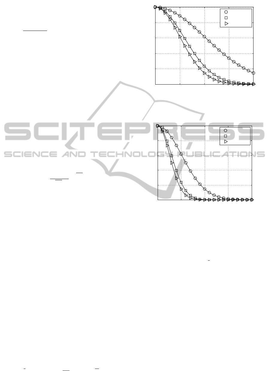
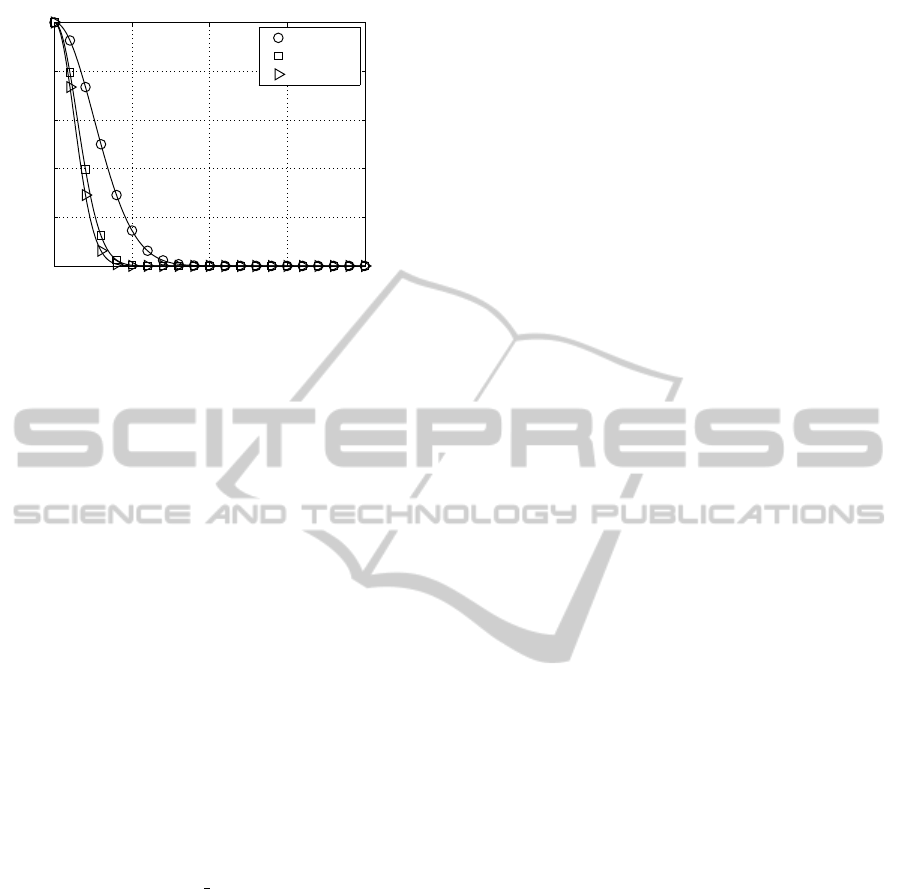
dispersion. It has been shown (see Fig. 3– 5) that the

correlation effect increases as the antennas’ separa-

tion diminishes. Furthermore, the correlation effect

diminishes as the departure angle increases. On the

other hand, the larger the spread angle the lower the

correlation coefﬁcient.

As the singular values decomposition is used to

pre- and post-processing of the system signals in or-

der to avoid inter-antenna interferences, the impact of

antennas correlation on the singular values has been

analysed (see Fig. 8–9). By applying the SVD, the

MIMO channel can be described as multiple indepen-

dent SISO channels (so called layers) with different

gains (given by the corresponding singular values).

For the same noise power at the receive antenna, the

larger the singular value the higher is the SISO chan-

nel reliability. The ideal situation is when all sin-

gular values are equal. The apparition of predomi-

nant layers (high valued singular value) is accompa-

nied by weak layers (low valued singular value). As

highlighted in Fig. 8 and 9, the difference between

the the smallest and the largest layer-speciﬁc singular

value becomes smaller as the antennas correlation in-

creases. The antennas correlation effect increases the

probability of having predominant layers.

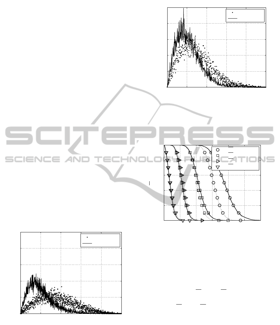
0 0.2 0.4 0.6 0.8 1

0.002

0.004

0.006

0.008

0.01

uncorrelated

correlated

pdf →

singular value →

Figure 8: PDF (probability density function) of the ratio ϑ

between the smallest and the largest singular value for cor-

related (solid line) as well as uncorrelated (dotted line) fre-

quency non-selective (2×2) MIMO channels (d

= 1/32,

φ = 30

◦

rad and σ

= 1,0).

In order to show the distribution of the layer-

speciﬁc characteristic properly, the CCDF (comple-

mentary cumulative distribution function) is used (see

0 0.1 0.2 0.3 0.4 0.5

0.002

0.004

0.006

0.008

0.01

uncorrelated

correlated

pdf →

singular value →

Figure 9: PDF (probability density function) of the ratio ϑ

between the smallest and the largest singular value for cor-

related (solid line) as well as uncorrelated (dotted line) fre-

quency non-selective (4×4) MIMO channels (d

= 1/32,

φ = 30

◦

rad and σ

= 1,0).

0 1 2 3 4 5 6

0.2

0.4

0.6

0.8

(1st layer)

(2nd layer)

(3rd layer)

(4th layer)

Prob{

ℓ

≥U} →

U →

Figure 10: CCDF of the layer-speciﬁc distribution for cor-

related (solid line) as well as uncorrelated (dotted line) fre-

quency non-selective (4×4) MIMO channels (d

= 1/32,

φ = 30

◦

rad and σ

= 1,0).

Fig. 10). It can be noticed the different effect on

strong and weak layers. The antennas correlation in-

creases the probability of having layers with larger

values (see layers

and

) and increases for

weak layers the probability of having lower values

(see layers

and

5 CONCLUSIONS

Due to the proximity of transmitter and receiver side

antenna arrays the theoretically possible potential of

MIMO is signiﬁcantly reduced by correlation. As

shown by computer simulations, under the effect of

correlation, the inﬂuence of layers with high weight-

ing factors becomes even stronger whereas the inﬂu-

ence of layer with low weighting factors diminished.

PECCS2013-InternationalConferenceonPervasiveandEmbeddedComputingandCommunicationSystems

154

Our results show that not necessarily all layers might

be used for the data transmission even when the wave-

propagation between the different pairs of transmit

and receive antennas is affected by correlation.

REFERENCES

Ertel, R., Cardieri, P., Sowerby, K. W., Rappaport, T. S.,

and Reed, J. H. (1998). Overview of Spatial Channel

Models for Antenna Array Communication Systems.

IEEE Personal Communications, 5(1):10–22.

Haykin, S. S. (2002). Adaptive Filter Theory. Prentice Hall,

New Jersey.

Laub, A. J. (2005). Matrix Analysis for Scientists and Engi-

neers. Society for Industrial and applied Mathematics,

Philadelphia.

Lee, W.-Y. (1973). Effects on Correlation between two Mo-

bile Radio Base-Station Antennas. IEEE Transactions

on Vehicular Technology, 22(4):130–140.

Oestges, C. (2006). Validity of the Kronocker Model for

MIMO Correlated Channels. In Vehicular Technology

Conference, volume 6, pages 2818–2822, Melbourne.

Salz, J. and Winters, J. H. (1994). Effect of Fading Correla-

tion on adaptive Arrays in digital Mobile Radio. IEEE

Transactions on Vehicular Technology, 43(4):1049–

1057.

Shiu, D., Foschini, G., Gans, M., and Kahn, J. (2000). Fad-

ing Correlation and its Effect on the Capacity of Mul-

tielement Antenna Systems. IEEE Transactions on

Communications, 48(3):502–513.

Taparugssanagorn, A., Jasma, T., and Ylitalo, J. (2006).

Spatial Correlation and Eigenvalue Statistics Investi-

gation of Wideband MIMO Channel Measurements.

In IEEE 17th International Symposium on Personal,

Indoor and Mobile Radio Communications (PIMRC),

pages 1–5.

Wang, H., Wang, P., Ping, L., and Lin, X. (2009). How

Does Correlation Affect the Capacity of MIMO Sys-

tems with Rate Constraints? In IEEE Global Telecom-

munications Conference (GLOBECOM), pages 1–5.

Yueyu, W. and Lili, G. (2007). Analysis on Spatial Corre-

lation Related with Antenna Array of MIMO System.

In International Conference on Wireless Communica-

tions, Networking and Mobile Computing (WiCom),

pages 456–459.

AnalysisofMIMOSystemswithTransmitter-sideAntennasCorrelation

155