
Continuous-time Revenue Management in Carparks
Part Two: Refining the PDE
Andreas Papayiannis, Paul Johnson, Dmitry Yumashev and Peter Duck
School of Mathematics, University of Manchester, Oxford Road, Manchester M13 9PL, U.K.
Keywords:
Expected Revenue, Rejection Policy.
Abstract:
In this paper, we study optimal revenue management applied to carparks, with the primary objective to max-
imize revenues under a continuous-time framework. This work is an extension to (Papayiannis et al., 2012)
where the authors developed a Partial Differential Equation (PDE) model that could solve for the rate at which
cash is generated through an infinitesimal time. However, in practice, carpark managers charge customers
per day or per hour which is a finite period of time. Unfortunately, this situation was currently not captured
by this previous work. Therefore, our current work attempts to reformulate the existing PDE in a way that
it does capture the revenue that is generated within any finite time interval of length ∆T. The new model is
compared against the Monte Carlo (MC) approach for several choices of ∆T; the results are remarkable as the
improvement in computation speed and efficiency are significant. Since, the algorithm in the PDE still does
not solve the ‘exact’ problem, a method is proposed to marry the benefits of the PDE with those of the MC
approach. Our results are prominent as the optimal values generated in this case have shown to be extremely
close to the MC ones while the computation times are kept to a minimum.
1 INTRODUCTION
The primary objectiveof this paper is to study revenue
management applied to carparks, in order to optimally
manage the expected revenues of the carpark under a
continuous time framework. There has been an in-
creasing interest on car parking problems within the
last two decades. Many researchers have worked on
traffic congestion problems, among them are (Teodor-
ovi´c and Vukadinovi´c, 1998), (Arnott and Rowse,
1999) and (Zhao et al., 2010), to just list a few. An
extensive review on urban car parking models can be
found in (Young et al., 1991). In the context of rev-
enue management we refer to (Teodorovi´c and Luˇci´c,
2006) who proposed an intelligent parking inventory
control system based on fuzzy logic theory. More-
over, (Onieva et al., 2011) have formulated and solved
a Linear Programming (LP) problem in both a de-
terministic and a stochastic environment. In this pa-
per, however, we aim to build upon the framework
laid down by (Papayiannis et al., 2012) and extend
the Partial Differential Equation (PDE) approach to a
more realistic discrete time framework. In (Papayian-
nis et al., 2012) the authors present two approaches
of modelling such a continuous-time stochastic opti-
mization problem; the Monte-Carlo (MC) approach
and the PDE approach. The first one solves the prob-
lem by first setting up the selling horizon and then
discretising the horizon into finite intervals of time
∆T. Bookings in both cases are modelled using fixed
time-invariant Poisson distribution for the number of
bookings with exponential waiting times for time be-
tween booking and length of stay exponential arrival
times have also been employed in (Onieva et al.,
2011; Teodorovi´c and Luˇci´c, 2006). The carpark is
then managed by assigning an accept/reject decision
to the bookings in each time interval given the cur-
rent state of the carpark (i.e. number of spaces re-
maining and time until stay). This decision was opti-
mally taken so that a parking slot never sells for less
than what we might expect to receive for it in the fu-
ture. For the PDE approach, the authors derive an-
alytical formulae for the probability distributions of
bookings so that they can formulate an expression for
the expected value of all the available spaces at time t
given we know the value of spaces remaining at time
t + dt. Since the process is essentially Markov they
can evoke the Hamilton-Jacobi-Bellman principle as
in (Gallego and van Ryzin, 1994) to express this as a
dynamic programming problem. The resulting PDE
was in fact solving for the rate at which the value is
generated through an infinitesimal time, rather than
over some discrete time as in the case of the Monte
Carlo method. Thus, a comparison on the optimal so-
274
Papayiannis A., Johnson P., Yumashev D. and Duck P..
Continuous-time Revenue Management in Carparks - Part Two: Refining the PDE.
DOI: 10.5220/0004219200760081
In Proceedings of the 2nd International Conference on Operations Research and Enterprise Systems (ICORES-2013), pages 76-81
ISBN: 978-989-8565-40-2
Copyright
c
2013 SCITEPRESS (Science and Technology Publications, Lda.)

lution between the MC and the PDE methodologies
could only be made in the limit i.e. as the time in-
tervals in the MC tend to zero ∆T → 0; the optimal
values however were showed to be remarkably close
to one another.
On the one hand, the pricing structure of most
carparks dictates that spaces are sold to customers
in slots, typically an integer number of fixed periods
of time, such as day or hour over which the space
will be reserved (see (Teodorovi´c and Luˇci´c, 2006;
Onieva et al., 2011)). On the other hand, (Bitran and
Caldentey, 2003) argue that “the explosive growth of
the Internet and e-commerce make the continuous-
time model much more suitable in practice”. More-
over, the results of (Papayiannis et al., 2012) have
shown the superiority of the PDE method over the
MC method with respect to both efficiency and com-
putational speed, but the PDE method presented there
could not capture discrete time intervals. These then
provide the motivation for the current study to ex-
tend the PDE model so that it can solve for the rate
at which value is generated within any time period of
finite size ∆T.
The remainder of this report is organized as fol-
lows. In section 2 we explain the steps taken in or-
der to reformulate the problem. Section 3 illustrates
some numerical results along with discussion. All re-
sults which are presented in this paper are obtained
using an Intel Xeon(R) CPU E5450 @3.00GHz with
16GB of RAM. Finally our conclusions can be found
in section 4.
2 PROBLEM FORMULATION
The derived PDE in (Papayianniset al., 2012) is based
on the probability densities P
s
and g which are used
to calculate the rate at which bookings turn up and
stay as of time t for the infinitesimal period T > t,
and the rate of cash-flow running through that period.
However, we note that the continuous time effect of
the PDE is on the booking decision rather than the
actual time spent in the carpark.
Therefore, we can still have the bookings arriv-
ing in a continuous-time but rather calculate the as-
sociated revenue rates within a discrete time inter-
val in the future, the size of which can be of any fi-
nite length ∆T. In other words, we can still consider
that bookings are made instantaneously but, also ad-
just the probability distributions in such a way that
we rather capture the probability of a customer being
present within the interval [T, T + ∆T] which takes
place between [τ, τ + ∆T] days after the booking is
made.
Now within the time-invariant framework, we in-
troduce ˜g(τ) (the symbol ‘∼’ will be used in the defi-
nitions throughout this report to distinguish the terms
that involve the finite interval ∆T) to be the fraction
of customers who made their bookings to be present
between τ and τ + ∆T days later. It is not difficult to
show that this may be written as
˜g(τ) = P
a
(τ+ ∆T) − P
d
(τ). (1)
Similarly, we introduce
˜
f(τ) to be the average inten-
sity for bookings made so that they are present be-
tween [τ, τ + ∆T] days later. This can be expressed
as
˜
f(τ) = λ
b
˜g(τ). (2)
Moreover, we define the probability density of a cus-
tomer staying ξ days given that he/she is present be-
tween [τ, τ + ∆T] days after the booking made by
˜
ρ
s
(ξ|τ) which can be expressed as,
˜
ρ
s
(ξ|τ) =
ρ
s
(ξ)[P
a
(τ+ ∆T) − P
a
({τ− ξ, 0}
+
)]
˜g(τ)
. (3)
It should be made clear at this stage that ρ
s
(ξ|τ) ⊆
˜
ρ
s
(ξ|τ).
Consequently, the cumulative probability of a cus-
tomer staying no more than ξ days given that he/she is
present between [τ, τ+∆T] after the booking,
˜
P
s
(ξ|τ),
is given by
˜
P
s
(ξ|τ) =
Z
ξ
0
˜
ρ
s
(s|τ)ds. (4)
It is important to mention that although we have
modified the probability distributions, the customers
are still booking in continuous time and request to
park for any length of stay which is again still a con-
tinuous quantity. For the case of maximising the cash-
flows within a finite time period, any bookings that
happen to be present at any time within this interval
do contribute to the solution. In (Papayiannis et al.,
2012) PDE model we looked at all bookings that are
present during the same infinitesimal and given that
bookings could only be distinguished by their length
of stay (the larger the length of stay, the less the price
to be paid per day) we imposed a rule to reject those
of length greater than ξ
∗
. In our new formation, the
idea is similar with the only difference that we are
now looking at all bookings that are present at any
time within a finite time interval. Unfortunately, this
increases the complexity of the problem as bookings
present in the same period, although being of same
length of stay, they might have pay a different price
rate according to how many time periods ∆T each
falls into in total (this depends on the exact time point
the bookings lie when being within the time period).
Therefore, we suggest a simple procedure to estimate
Continuous-timeRevenueManagementinCarparks-PartTwo:RefiningthePDE
275
the number of time periods (n) for which the cus-
tomers are likely to occupy the slot, which will in turn
enable us to determine a better estimate for the price
rates that should be applied. We note that n should
strongly depend on the size of the time period, ∆T.
In particular, we assume that the required length
of stay ξ is between k and k + 1 times larger than the
length of the interval ∆T, i.e. k∆T ≤ ξ ≤ (k + 1)∆T,
where k ∈ Z. For simplicity, we assume that cus-
tomers arrival times follow a uniform distribution, u.
Figure 1 illustrates the situation; In order for cus-
tomers who stay for ξ days to be accounted within the
time interval [T, T + ∆T], they must have arrived no
more that ξ days in advance and no later than T + ∆T.
Thus the feasible region, within which customers con-
tribute to the solution, is T − ξ ≤ t ≤ T + ∆T. There-
fore, the uniform distribution’s endpoints become 0 ≤
u ≤ ∆T + ξ.
Regarding the number of periods (n) the cus-
tomers are likely to occupy a slot for, there are only
two possible scenarios;
1. the customer stays k+ 1 periods when his/her re-
quired duration of stay covers k periods plus a
fraction of an additional period either before or
after this interval (his/her arrival time lies on a red
segment of figure 1),
2. or stays k + 2 periods when his/her then required
duration of stay covers the same k periods plus a
fraction before and after this interval (his/her ar-
rival time lies on a green segment of figure 1).
In particular, we can show that the associated proba-
bility in each case is given by,
P(n = k + 1) = (k+ 1)
(k+ 1)∆T − ξ
ξ+ ∆T
(5)
while,
P(n = k + 2) = 1− P(n = k + 1) (6)
Therefore, n is given by
n =
k+ 1 w.p P
1
= (k+ 1)
(k+1)∆T−ξ
ξ+∆T
k+ 2 w.p P
2
=
(k+2)ξ−
(
1−(k+1)
2
)
∆T
ξ+∆T
Consequently, the expected length of stay (E[n])
becomes
E[n] = (k+ 1)P
1
+ (k+ 2)P
2
. (7)
Finally, we can replace the exact duration of stay,
ξ, by the expected number of time periods (of length
∆T) the customer is staying for, E[n], and then we can
calculate the required price rate per period as,
Ψ(ξ) →
˜
Ψ(E[n]) ≡ ψ
1
+ ψ
2
e
−µE[n]∆T
. (8)
Figure 1: Uniform arrival distribution u(0, ∆T + ξ) for cus-
tomers that stay for k∆T ≤ ξ ≤ (k + 1)∆T days and they
are present within the interval [T, T + ∆T]. Customers who
arrive anywhere on the red segments will occupy k+1 inter-
vals while those that arrive anywhere on the green segments
will occupy k + 2 intervals.
6
8
10
12
14
0 1 2 3 4 5 6 7 8 9 10
Price Rate
ξ
Continuous
Adjusted (∆T=1.0)
Jump (∆T=1.0)
6
8
10
12
14
0 1 2 3 4 5 6 7 8 9 10
Price Rate
ξ
Continuous
Adjusted (∆T=0.5)
Jump (∆T=0.5)
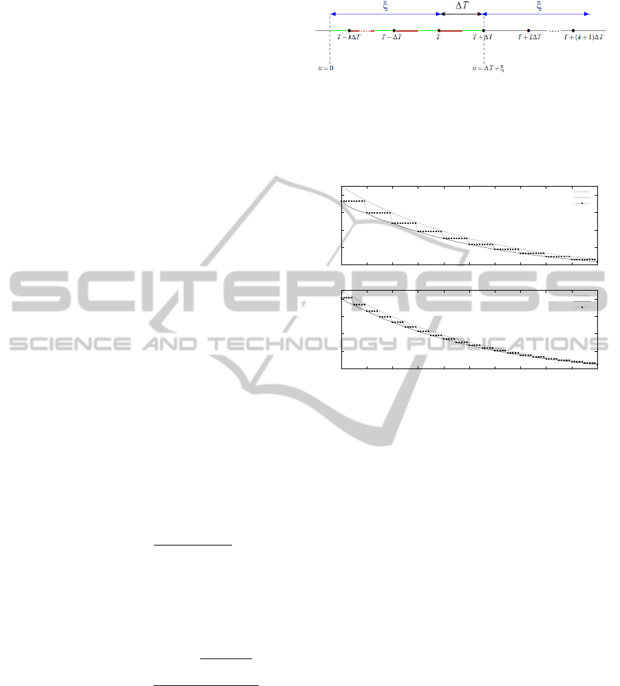
Figure 2: Plots of the adjusted price rate function used in
the reformulated PDE and the discrete-jump price func-
tion used in the MC. Upper figure compares the two for
∆T = 1.0 while the lower figure plots these for ∆T = 0.5.
The continuous pricing function (as in (Papayiannis et al.,
2012)) is shown as well.
with parameters ψ
1
, ψ
2
, µ identical to those in (Pa-
payiannis et al., 2012). Figure 2 compares the ad-
justed price rate function (8) with the corresponding
discrete-jump price function that has been used in the
MC; the upper figure illustrates this comparison for
∆T = 1.0 while the lower figure for ∆T = 0.5. In
each figure the continuous pricing function (as in (Pa-
payiannis et al., 2012)) is plotted as well. The ad-
justed price rate function seems a reasonable approx-
imation to the discrete-jump price function; the two
functions approach one another as ∆T decreases and,
in fact, they become equal in the limit (as ∆T → 0).
In the limiting case both pricing functions are equal
to the continuous pricing function (8). Finally, we
define
˜
V(Q, t;T) to the rate at which revenue is gen-
erated in the carpark with Q spaces remaining for the
future period [T, T + ∆T] as of time t. Thus, within
the time-invariant framework we may define
˜
V(Q, τ)
as the rate at which revenue is generated from cars
present over the period interval which is formed be-
tween [τ, τ+ ∆T] days later.
ICORES2013-InternationalConferenceonOperationsResearchandEnterpriseSystems
276

Therefore, the modified PDE can be written as
∂
˜
V
∂τ
= max
ξ
∗
˜
P
s
(ξ
∗
|τ)
˜
f(τ)(
˜
V(Q− 1, τ) −
˜
V(Q, τ))
+
˜
f(τ)
Z
ξ
∗
0
˜
ρ
s
(ξ|τ)
˜
Ψ(ξ)dξ
, (9)
with the same boundary conditions as before
˜
V = 0 when τ = 0 (10)
˜
V = 0 when Q = 0. (11)
The solution to this system gives the rate at which the
value is generated in the future time period [T, T +
∆T] which takes place between τ and τ+ ∆T days af-
ter the current time t and the values ξ
∗
= ξ
∗
(Q, τ) that
achieve the supremum construct the optimal rejection
policy
1
.
The optimal rejection policy can alternatively be
expressed in terms of the ‘Added Values’ of the
spaces (Papayiannis et al., 2012); in particular the op-
timal policy satisfies
˜
Ψ(ξ
∗
) =
˜
V(Q, τ) −
˜
V(Q− 1, τ) ∀Q ∀τ.
In the revenue management literature this quantity is
usually referred to as the opportunity cost of selling
a unit of capacity when the time left is τ and the
available inventory is Q, or simply as the expected
marginal value of capacity at time τ (see (Talluri and
van Ryzin, 2004)).
3 NUMERICAL RESULTS
3.1 Numerical Solution of the PDE
In this section we present some numerical results to
compare the PDE scheme in (9) with the MC ap-
proach
2
. We have used a time horizon T = 30 and
carpark capacities 1 ≤ Q ≤ 100. Regarding the book-
ing patterns, we use exponential distributions with
constant intensities and two distinct booking classes
as in (Papayiannis et al., 2012).
Below, we present the expected revenues gener-
ated within the period [T, T + ∆T] as of time t = 0,
calculated by the MC approach first and then from our
adjusted PDE scheme. By assuming time-invariance,
1
Note that the optimal durations ξ
∗
are now applied to
entire period intervals of length ∆T.
2
In the MC approach we obtain the correct solution us-
ing an iteration scheme for which the number of paths (sim-
ulations) increase in each iteration. The iterations terminate
once the frobenious norm is minimised and the converged
solution forms the optimal solution.
0
100
200
300
400
500
600
0 5 10 15 20 25
Expected Revenues
Time Left, τ
MC- Expected Revenues (Q=50)
∆T=1.0
∆T=0.5
∆T=0.25
∆T=0.125
Figure 3: Expected Revenues using the MC approach as a
function time left τ. The capacity is fixed to Q = 50 and the
finite period is allowed to vary, ∆T = 1.0, 0.5, 0.25, 0.125.
0
100
200
300
400
500
600
0 5 10 15 20 25
Expected Revenues
Time Left, τ
PDE- Expected Revenues (Q=50)
∆T=1.0
∆T=0.5
∆T=0.25
∆T=0.125
Figure 4: Expected Revenues using the reformulated PDE
as a function time left τ. The capacity is fixed to
Q = 50 and the finite period is allowed to vary, ∆T =
1.0, 0.5, 0.25, 0.125.
these can be interpreted as the value of the carpark
with capacity Q as of [τ, τ + ∆T] time before all re-
maining spaces must be occupied. Figure 3 shows
results from the MC approach when the capacity is
50 and ∆T is allowed to change, while figure 4 shows
the corresponding results using the PDE method. The
expected revenues of the two approaches are remark-
ably close to each other for all choices of ∆T. De-
spite its simplicity, the PDE in (9) proves capable
of approximating the revenues, as these are derived
from the MC approach, for any given ∆T. We notice
that the expected revenues increase as the time left
increases; this implies that as the selling horizon in-
creases the carpark manager faces a larger population
of potential customers and therefore he/she can tar-
get the available capacity to the most lucrative ones
(see (Bitran and Caldentey, 2003), (Gallego and van
Ryzin, 1994)). In addition, the expected revenues in-
crease as ∆T increases; this is because when the pric-
Continuous-timeRevenueManagementinCarparks-PartTwo:RefiningthePDE
277

Table 1: Computation Times and Convergence for the MC
approach.
∆T # of Paths Iterations Comput. Times
1.0 12672 15 126.7s
0.5 25342 17 325.8s
0.25 35839 18 621.1s
0.125 50683 19 1334.6s
ing policy of the carparks management is to sell the
slots per day rather than per hour, for instance, a cus-
tomer is forced to pay the price rate for the entire
day even though he/she might only be staying for one
hour.
Table 1 illustrates the statistics obtained in the pro-
cess of calculating the entire set of optimal values (the
entire matrix for all capacities and times). The results
in table 1 indicate that the MC method (on its own)
is infeasible in practice; for carparks that operate with
slots that can be booked for a minimum of 3 hours
(∆T = 0.125) the MC approach is very poor as a cus-
tomer would have to wait an unrealistically long time
(more than 22 minutes!) until a decision would be
made as to whether he/she is allowed to park or not.
In the PDE, the time it takes to obtain the optimal so-
lution is tiny (never more than 25 seconds) and it does
not depend on ∆T at all. That it is independent of ∆T
means that the PDE meets the needs of any carpark-
ing management since it fits to any given price policy,
while the speed advantage of the PDE over the MC
renders it ideal for being used in a web reservation
engine.
However, in accordance to (Papayiannis et al.,
2012) the PDE in (9) generates slightly higher rev-
enues as it still does not solve the ‘exact’ problem; the
optimal decision algorithm still looks at each booking
length as separate days and solves for each day indi-
vidually, whereas in the MC approach the rejection al-
gorithm regards each request as a ‘group’ of days and,
thus, the optimal decision is based on the entire book-
ing length with a booking being accepted/rejected as
a whole (which is the situation in a real carpark).
Therefore, to exploit the speed advantage of the PDE
while preserving the correct optimisation algorithm
(of the MC approach) the PDE could be used jointly
with a Monte-Carlo method.
3.2 Using the PDE and MC Methods
Jointly
The MC approach in section 3.1 did calculate the op-
timal solution to the ‘exact’ problem in question but it
failed to do that in a reasonable time; table 1 showed
the large number of iterations and paths required for
the MC approach to converge to the optimal solution.
By contrast, the PDE methodology (9) calculated the
optimal solution in significanlty less time but this so-
lution did not correspond to the ‘exact’ problem; the
optimal decision was found after solving for each pe-
riod of day individually whereas in the MC the opti-
mal solution takes into account the inter-dependence
within days see (Papayiannis et al., 2012). Therefore,
our aim is develop a new improved methodology that
combines the best elements of the PDE (speed and ef-
ficiency) with the best ones of the MC (correct rejec-
tion algorithm that regards each request as a ‘group’
of days).
The ‘Joint’ Method. The optimal rejection policy
(‘Added Values’) is derived using the PDE in (9).
Then, this policy is employed in a Monte-Carlo pro-
cedure, where booking simulations are taken and re-
quests are allowed/denied service as a ‘group’. The
expected revenues are approximated by averaging
over ten thousand paths. We note that this procedure
does not require any iterations, as the optimal rejec-
tion policy would have already been derived by the
PDE. The results are recorded and compared against
the true results that have previously been calculated
by running the MC approach solely.
0
100
200
300
400
500
600
0 5 10 15 20 25
Expected Revenues
Time Left, τ
Joint PDE and MC- Expected Revenues
∆T=1.0
∆T=0.5
∆T=0.25
∆T=0.125
Figure 5: Expected Revenues using the joint approach as a
function time left τ. The capacity is fixed to Q = 50 and the
finite period is allowed to vary, ∆T = 1.0, 0.5, 0.25, 0.125.
Figure 5 shows the expected revenues generated
by the ‘joint’ method when Q = 50 as functions of
time, for varying time intervals ∆T. It is clear that
the curves are now outstandingly close to those in
figure 3. Table 2 is provided in regards to the max-
imum relative percentage errors obtained (by consid-
ering all τ) for different carpark sizes and different
time intervals ∆T. from this one may notice that the
maximum relative error decreases with the size of the
interval ∆T. Indeed, this is the case because the opti-
mal policy comes from the PDE scheme and we know
that the PDE solution converges to the MC solution
ICORES2013-InternationalConferenceonOperationsResearchandEnterpriseSystems
278

Table 2: Relative (%) Errors for varying capacities.
∆T
Capacity, Q
10 20 40 60 80
1.0 6.67 3.15 1.68 0.91 0.55
0.5 1.83 0.64 0.48 0.51 0.51
0.25 1.58 1.17 1.46 1.46 1.46
0.125 1.65 0.87 0.58 0.58 0.58
Table 3: Computation Times for the ‘joint’ method.
∆T Comput. Times Relative Comput. Times
1.0 45.5s 46.7%
0.5 56.8s 17.5%
0.25 71.6s 11.5%
0.125 102.4s 7.7%
as ∆T → 0. To justify this further the reader is re-
ferred to figure 2 where it shows that the price rate
functions used in the two methods would converge
as ∆T → 0. Moreover, the maximum relative error
decreases with capacity. This observation has more
to do with the nature of the carpark rather than the
choice of the method, as relatively big carparks might
require little or even no optimization at all, which im-
plies that the role of any optimal policy is reduced and
thus both methods would be even closer to each other.
Lastly, table 3 presents the computation times needed
for the ‘joint’ method to calculate the full set of opti-
mal revenues (the entire matrix for all capacities and
times) along with a relative speed comparison against
the MC approach. Our results show that the reduction
in computation time is significant; in particular, for
∆T = 1, the ‘joint’ algorithm takes only 46% of the
time it would take the MC approach to calculate the
optimal solution. When ∆T = 0.125 the statistics are
even more impressive as it only needs less than 8% of
the original time. This monotonic increase in speed
is explained by the fact that the time the PDE takes
to calculate the optimal policy is independent of the
size of ∆T, while in the MC the computation times
increase linearly.
4 CONCLUSIONS
In this paper, we have worked with the continuous-
time PDE model and MC model proposed in (Pa-
payiannis et al., 2012). Since the PDE could only
solve for the rate at which cash is generated through
an infinitesimal time we reformulated it in such a way
that it solves for the cash that is generated within a
time period of finite size ∆T and matched that against
the MC. The results validated our expectations as the
optimal values and optimal rejection policies where
remarkably close to one another. Moreover, the opti-
mal surfaces from the reformulated PDE where much
smoother and the computation times have improved
significantly. However, as the PDE could still not
solve the ‘exact’ problem we have proposed a ‘joint’
method that calculates the optimal policy from the
PDE and it then employs this to make optimal deci-
sions by using the MC. This method performed ex-
ceptionally well as it produced revenues around 1%
of the actual ones at most cases. For carparks that op-
erate with slots that can be booked for a minimum of
3 hours (∆T = 0.125) the improvement in computa-
tional speed was more than 92% (it only took 7.7% of
the original time) which it renders it ideal for being
used in a web reservation engine; for even smaller ∆T
the speed improvement is expected to be greater.
REFERENCES
Arnott, R. and Rowse, J. (1999). Modeling parking. Journal
of Urban Economics, 45(1):97 – 124.
Bitran, G. and Caldentey, R. (2003). An overview of pricing
models for revenue management. Manufacturing and
Service Operations Management, 5(3):203 – 229.
Gallego, G. and van Ryzin, G. (1994). Optimal dynamic
pricing of inventories with stochastic demand over fi-
nite horizons. Management Science, 40(8):pp. 999–
1020.
Onieva, L., Mu˜nuzuri, J., Guadix, J., and Cortes, P. (2011).
An overview of revenue management in service indus-
tries: an application to car parks. The Service Indus-
tries Journal, 31(1):pp.91–105.
Papayiannis, A., Johnson, P., Yumashev, D., Howell, S.,
Proudlove, N., and Duck, P. (2012). Continuous-
time revenue management in carparks. In Proceed-
ings of the 1st International Conference on Opera-
tions Research and Enterprise Systems, pages 73–82.
ICORES, SciTePress Digital Library.
Talluri, K. and van Ryzin, G. (2004). The Theory and Prac-
tice of Revenue Management. Kluwer Academic Pub-
lishers, Boston/Dordrecht/London.
Teodorovi´c, D. and Luˇci´c, P. (2006). Intelligent parking
systems. European Journal of Operational Research,
175(3):1666 – 1681.
Teodorovi´c, D. and Vukadinovi´c, K. (1998). Traffic con-
trol and Trasport Planning: A Fuzzy Sets and Neural
Netweorks Approach. Kluwer Academic Publishers,
Boston.
Young, W., Thompson, R. G., and Taylor, M. A. (1991). A
review of urban car parking models. Transport Re-
views, 11(1):63–84.
Zhao, Y., Triantis, K., Teodorovic, D., and Edara, P. (2010).
A travel demand management strategy: The down-
town space reservation system. European Journal of
Operational Research, 205(3):584 – 594.
Continuous-timeRevenueManagementinCarparks-PartTwo:RefiningthePDE
279
