
Linear Subspace Learning based on a Learned Discriminative
Dictionary for Sparse Coding
Shibo Gao
1
, Yizhou Yu
2
and Yongmei Cheng
1
1
College of Automation, Northwestern Polytechnical University, Xi’an, China
2
Department of Computer Science, The University of Hong Kong, Hong Kong, Hong Kong
Keywords: Face Recognition, Linear Subspace Learning, Discriminative Dictionary Learning.
Abstract: Learning linear subspaces for high-dimensional data is an important task in pattern recognition. A modern
approach for linear subspace learning decomposes every training image into a more discriminative part
(MDP) and a less discriminative part (LDP) via sparse coding before learning the projection matrix. In this
paper, we present a new linear subspace learning algorithm through discriminative dictionary learning. Our
main contribution is a new objective function and its associated algorithm for learning an overcomplete
discriminative dictionary from a set of labeled training examples. We use a Fisher ratio defined over sparse
coding coefficients as the objective function. Atoms from the optimized dictionary are used for subsequent
image decomposition. We obtain local MDPs and LDPs by dividing images into rectangular blocks,
followed by blockwise feature grouping and image decomposition. We learn a global linear projection with
higher classification accuracy through the local MDPs and LDPs. Experimental results on benchmark face
image databases demonstrate the effectiveness of our method.
1 INTRODUCTION
Linear subspace learning (LSL) is a popular method
for dimensionality reduction and feature extraction
for many pattern recognition tasks, including face
recognition (Cai et al., 2007, Huang et al., 2011, Lu
et al., 2010). It typically learns an optimal subspace
or linear projection according to a task-driven
criterion. High-dimensional data can be linearly
reduced to lower-dimensional subspaces through
LSL. Usually, recognition performance can be
improved in such lower-dimensional subspaces (Cai
et al., 2007).
There are both unsupervised and supervised LSL
methods according to whether they exploit the class
label information of train data. Representative
techniques of the two classes of LSL methods are
Eigenface (Turk et al., 1991) and Fisherface
(Belhumeur et al., 1997), respectively. The
corresponding algorithms are Principal Component
Analysis (PCA), and Linear Discriminant Analysis
(LDA). PCA seeks an optimal subspace with
maximal variances while LDA looks for a linear
combination of features which characterize or
separate two or more classes of objects. A
supervised LSL method that utilizes the label
information can usually obtain a better
discriminative subspace for classification problems.
Many supervised LSL methods have been proposed
as variants of LDA, including regularized LDA
(RLDA) (Lu et al., 2005), and perturbation LDA
(PLDA) (Zheng et al., 2009). As shown in (Zheng et
al., 2009), both of LDA and RLDA share an
assumption that the class empirical mean is equal to
its expectation. This assumption may not be valid in
practice and a new algorithm, called perturbation
LDA (PLDA), is developed. In the algorithm,
perturbation random vectors are introduced to learn
the effect of the difference between the class
empirical mean and its expectation under the Fisher
criterion. When the number of training samples is
less than the dimensionality of a sample, the within-
class scatter matrix in LDA becomes singular, and
PCA is often used to reduce the dimensionality
before LDA. In (Zheng et al., 2005) a GA-Fisher
method is proposed to select the eigenvectors
automatically in PCA before LDA. In (Qiao et al.,
2009) a sparse LDA is presented to overcome the
small sample problem. In (Ji et al., 2008), the
authors present a unified framework for generalized
LDA via a transfer function.
A common goal shared among existing LSL
530
Gao S., Yu Y. and Cheng Y..
Linear Subspace Learning based on a Learned Discriminative Dictionary for Sparse Coding.
DOI: 10.5220/0004207905300538
In Proceedings of the International Conference on Computer Vision Theory and Applications (VISAPP-2013), pages 530-538
ISBN: 978-989-8565-47-1
Copyright
c
2013 SCITEPRESS (Science and Technology Publications, Lda.)

methods is that the learned subspace should be as
discriminative as possible. However, every image is
a superposition of both discriminative and non-
discriminative information. Most existing LSL
methods estimate the scatter matrices directly from
the original training samples or images. The non-
discriminative information in such training samples,
such as noise and trivial structures, may interfere
with discriminative subspace learning. Different
from most existing LSL methods, such as PCA,
FLDA/RLDA, LPP and SPP, where the subspace is
learned for image decomposition, a new LSL
framework is presented in (Zhang et al., 2011) to
perform image decomposition for subspace learning.
Dictionary learning and sparse coding are used for
adaptive image decomposition during the learning
stage, where the image is decomposed and the image
components are used for guiding subspace learning.
With the development of l
0
- and l
1
-minimization
techniques, sparse coding and dictionary learning
have received much attention recently. The
dictionary learned in (Zhang et al., 2011) is a
generative or reconstructive dictionary which only
minimizes reconstruction errors. The atoms of the
dictionary do not necessarily have sufficient power
to discriminate among data with different class
labels. Thus, selecting the most discriminative atoms
from such a dictionary as in (Zhang et al., 2011)
may not achieve the full potential of sparse coding.
On the other hand, several methods have been
developed to represent discriminative information
during dictionary learning. A discriminative term
based on LDA is integrated into the classical
reconstructive energy formulation of sparse coding
in (Huang et al., 2007, Rodriguez et al., 2008).
However, a predefined dictionary instead of a
learned dictionary is used in (Huang et al., 2007). In
(Yang et al., 2011), a discriminative dictionary is
learned based on an objective function combining a
variant of Fisher criterion and a reconstruction error.
A potential problem with such an approach is that
the reconstruction error term may interfere with the
Fisher criterion and reduce its power when learning
a discriminative dictionary. A formulation of the
classification error of a linear SVM has also been
incorporated into dictionary learning (Jiang et al.,
2011, Zhang et al., 2010). Other efforts along this
direction include multi-class dictionary optimization
for gaining discriminative power in texture analysis
(Mairal et al., 2008). A compact dictionary is
learned from affine-transformed input images to
increase discriminative information (Kulkarni et al.,
2011). In (Mairal et al., 2012) a task-driven
supervised dictionary learning method is proposed
where dictionary learning relies on a subgradient
method to perform a nonconvex optimization. Note
that learning discriminative dictionaries based on the
SVM error term is not well suited for problems that
involve image patches because even images from
different classes may share similar patches, whose
class labels would be very hard to determine.
In this paper, we present a new linear subspace
learning method based on sparse coding using a
novel technique for discriminative dictionary
learning. We use a Fisher ratio defined over sparse
coding coefficients as the objective function for
optimizing a discriminative dictionary while the
condition that the sparse coding coefficients should
minimize the reconstruction error is imposed as a
constraint. Atoms that can achieve a higher Fisher
ratio of the sparse coding coefficients are considered
better. Therefore, discriminative information is
emphasized during the atom construction process. In
our decomposed image, the more discriminative part
(MDP) has a larger fisher ratio than the one obtained
from a reconstructive dictionary. We further obtain
local MDPs and LDPs by dividing images into
rectangular blocks, followed by blockwise feature
grouping and image decomposition. A more
effective global MDP and LDP can be obtained by
concatenating these local MDPs and LDPs. We learn
a global linear projection with higher classification
accuracy through the global MDPs and LDPs.
Experimental results on benchmark face image
databases demonstrate the effectiveness of our
method. The flowchart of the proposed LSL method
is shown in Fig. 1.
Figure 1: The flowchart of the proposed method.
2 IMAGE DECOMPOSITION
AND RECONSTRUCTION VIA
SPARSE CODING
The sparse representation model is a modern method
for image decomposition and reconstruction, which
have been used in many image-related applications,
such as image restoration and feature selection. The
sparse representation of a signal over an over-
complete dictionary is achieved by optimizing an
objective function that includes two terms: one
LinearSubspaceLearningbasedonaLearnedDiscriminativeDictionaryforSparseCoding
531

measures the signal reconstruction error and the
other measures the coefficients’ sparsity (Huang et
al., 2007). Suppose that the data
12
,,, R
mn
n
xx x
X
(n is the number of
samples, m is the number of dimensions) admits a
sparse approximation over an over-complete
dictionary
12
,,, R
mK
K
dd d
D
(with K>m)
with K atoms. Then X can be approximately
represented as a linear combination of a sparse
subset of atoms from D. The over-complete
dictionary D can be obtained by solving the
following optimization problem:
1
2
,
1
arg m in
in
i
i
n
ii
F
i
x
D
D
,
0
..
i
st
, where
i
is a
sparse coefficient vector, and each column of D is an
atom represented as a unit vector. In practice, the l
1
norm replaces the l
0
norm during optimization, that
is,
1
2
1
,1
arg min
in
i
i
n
ii i
F
i
x
D
D
(1)
The weight
controls the trade-off between the
reconstruction accuracy and the sparseness of the
coefficient vectors. The cost function given above is
non-convex with respect to both D and
i
.
However, it is convex when one of them is fixed.
Thus, this problem can be approached by alternating
between learning D while fixing
i
and inferring
i
while fixing D. We can see that a data sample x can
be decomposed into
1
()
K
k
k
x
kd
D
. If the
sparse coefficient vector
for the data item x is
known under the dictionary D, then the pre-image
can be reconstructed by
ˆ
x
D
. The sparse
coefficient vector
and the dictionary D contain the
most information about the data item x, therefore,
they have been used for tasks such as recognition,
feature extraction and image restoration.
3 DISCRIMINATIVE
DICTIONARY LEARNING
In this section, we introduce a new objective
function and its associated algorithm for learning an
overcomplete discriminative dictionary from a set of
labeled training image patches. Supervised
dictionary learning for achieving a goal other than
data reconstruction has proven to be a hard problem,
especially when the objective function for dictionary
learning is not differentiable everywhere in l
1
norm
restraint. Our algorithm relies on the subgradient
method to obtain optimized atoms. One of the key
contributions of our work is to train a discriminative
dictionary for subsequent feature grouping.
Note that Fisher’s criterion is motivated by the
intuitive idea that data samples from multiple classes
are maximally separated when samples from
different classes are distributed as far away from
each other as possible and samples from the same
class are distributed as close to each other as
possible. Because of the reconstructive capability of
an over-complete dictionary, the degree of
separation among data samples can be indicated by
the degree of separation among the sparse
coefficient vectors coding the data samples using the
dictionary. Thus, discriminative components of data
samples can be discovered by seeking a dictionary
whose corresponding sparse coefficient vectors
achieve a high Fisher’s ratio. Therefore, we use the
Fisher’s ratio defined over the sparse coefficient
vectors as the objective function for learning a
discriminative dictionary.
Let
R
m
i
x
(
1, 2, ,
k
C
in
) be a training
sample, an m-dimensional vector formed by image
patches of size
mm from images in the
k
C -th
class,
k
C
n
is the number of training samples in the
k
C -th class. The Fisher’s criterion is defined as
BW
F
isher x tr x tr x SS
, where
W
x
S
is
the within-class scatter matrix,
B
Sx
is the between-
class scatter matrix, which are defined as
1
mm
C
k
ik
n
T
Wikik
xC
kCi
xxx
S
and
mmmm
k
T
BCkk
kC
xn
S
, where m
k
is
the mean of training samples in class
k
C , and m is
the mean of all training samples. We can see that
BW
F
isher x tr x tr x SS
=
2
2
1
mm m
C
k
k
ik
n
Ck i k
F
F
xC
kC kCi
nx
.
Based on the Fisher’s criterion, we define
discriminative dictionary learning as follows:
2
α
1
2
αμ
arg min α (, )
μμ
C
k
ik
k
n
ik
F
C
kCi
Ck
F
kC
Jx
n
D
D
(2)
s.t.
2
1
α
α (, ) argmin αα
ii
F
xx
DD
where
α (, )
i
x
D
represents the optimal sparse
coefficient vector coding the training sample x using
VISAPP2013-InternationalConferenceonComputerVisionTheoryandApplications
532

the learned dictionary D,
1
1
μα
C
k
k
k
n
ki
i
C
iC
n
is the
mean sparse coefficient vector for training samples
in class
k
C ,
1
1
μα
n
k
k
n
is the mean sparse
coefficient vector,
k
C
kC
nn
is the total number of
training samples. Obviously, the numerator of the
above objective function,
2
α
1
αμ
C
k
ik
n
ik
F
C
kCi
,
represents the intra-class compactness, and the
denominator,
2
μμ
k
Ck
F
kC
n
, represents the inter-
class separability. Note that
α 1 α (x, )Fisher J
D
is the Fisher’s ratio
defined over the optimal sparse coefficient vectors.
So
min α (x, ) max αJFisher
D
. Note that
in the optimization defined in equation (2), the
discriminative Fisher ratio and the reconstruction
term are separated, one as the objective function and
the other as the constraint. Such a scheme guarantees
that there is least interference between the two and
the power of the Fisher criterion is fully realized.
Our method learns an entire discriminative
dictionary from labeled training data using the
Fisher criterion. The optimal sparse coefficient
vector of a training sample is actually a function of
dictionary D due to
2
1
α
α (, ) argmin αα
ii
F
xx
DD
. Therefore,
dictionary D is the only variable of the objective
function
α (, )Jx
D
. We will use ()F
D
as a short
notation in place of
α (, )Jx
D
when necessary. In
(Boureau et al., 2010, Mairal et al., 2012, Yang et al.,
2010), the subgradient method was used to optimize
functions of
α (, )
i
x
D
with respect to D (see the
APPENDIX). In our problem, the subgradient of
()F
D
with respect to D can in turn be computed
using the chain rule
**
*
α
α
()
α
i
i
i
TT
ii i i i
i
TT
J
F
x
D
DD
DD
DΒΑ XDAΒ
(3)
where
12 1
α , α , α , α ,,α R
kk
k
k
K
n
CC
C
A
,
12 1
=,, , ,, R
kk
k
k
Kn
CC
C
B
,
i
is
composed from
,
i
i
and
,
C
i
i
.
1
,,
,
,
( α )
=
α
T
i
iii
i
i
i
J
DD
,
,
0
C
i
i
, where
,
1, , : α 0
i
i
jKj
is the active set,
denoting the indices of the nonzero coefficients
within the sparse vector
α (, )
i
x
D
, and
,
1, , : α 0
C
i
i
jKj
is the non-active
set. Since
2
α
1
2
αμ
μμ
α
αα
C
k
ik
k
n
ik
F
C
kCi
Ck
F
kC
i
ii
n
J
2
α
1
22
2
αμ
2 αμ
2 μμ
μμ
μμ
C
k
ik
k
k
n
ik
F
ik
C
kCi
k
Ck
F
kC C k
F
kC
n
n
(4)
We have
1
,,
,
,
2
,
2
,
1
α
2
,
2
,
=
2 αμ
μμ
αμ
2 μμ
μμ
k
C
k
ik
k
T
iii
i
ik
i
Ck
i
F
kC
n
ik
i
F
kCi
C
k
i
Ck
i
F
kC
n
n
DD
(5)
In summary, the subgradient of
()F
D
at D can be
computed as
*TT
GDΒΑ XDAΒ
(6)
Since the subgradient method can obtain a search
direction at a certain point during optimization, it
can be used in convex, quasiconvex and nonconvex
problems (Burachik et al., 2010, Neto et al., 2011,
Yang et al., 2010). Here the dictionary D can be
updated by the subgradient G. That is
(1)
() ( 1)
(1)
t
tt
t
t
F
G
DD
G
(7)
where
t
is a learning rate, t is the current iteration
step. The step size of the learning rate should be
chosen carefully. In this paper, the learning rate
t
is
calculated from
0
1
t
tT
, where
0
is the
initial learning rate,
t
is the current learning rate,
LinearSubspaceLearningbasedonaLearnedDiscriminativeDictionaryforSparseCoding
533
T
is a predefined parameter, and the initial
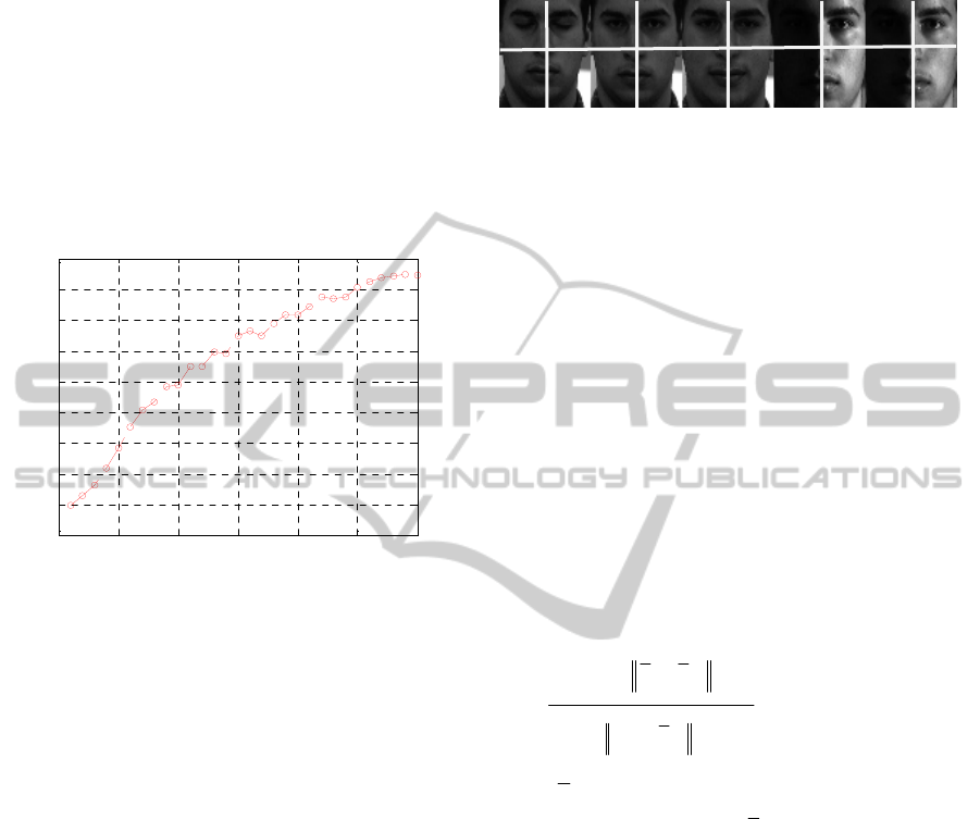
dictionary is learned using equation (1). Figure 2
shows the Fisher ratio versus the number of
iterations on image patches from the CMU PIE
database. We can see that the subgradient-based
optimization is a process with oscillatory
convergence.
Once the dictionary
D has been learned, a data
sample can be decomposed into components using
the atoms in
D as follows,
,1 , 2 ,
j
jj j jK
x
xx x
D
, where
,jk j k
x
kd
Figure 2: Fisher ratio versus the number of iterations on a
subset of the CMU PIE database.
4 LSL VIA DISCRIMINATIVE
DICTIONARY LEARNING
AND BLOCKWISE
DECOMPOSITION
4.1 Patch-based Dictionary Learning
The relatively high dimensionality of an image as
well as the usual relatively small number of training
images prevent us from learning a redundant
dictionary directly from a set of training images
under the sparse coding framework. Same to (Zhang
et al., 2011), a patch-based scheme is used to learn a
dictionary. As mentioned above, the defined
objective function (3) is very fit for patch-based
discriminative dictionary learning. Each training
image I
i
is partitioned into overlapping patches. The
complete set of patches from all training images is
denoted as
X=[x
1
, x
2
, …,x
n
], in which h is the total
number of patches. A discriminative dictionary is
learned from T following the optimization
framework presented in the previous section. Each
patch t
j
can be reconstructed through the atoms in the
learned dictionary as follows,
12
(1) (2) ( )
j
jj j j K
x
dd Kd
D
.
Figure 3: Partition of training images into blocks.
4.2 Blockwise Feature Grouping
We also partition an image I
i
into relatively large
blocks and perform blockwise feature grouping. Note
that each block includes multiple image patches. If an
image is divided into L blocks, for each patch
l
j
x
in
block l,
,
11
()
KK
ll l l
j
jjkjk
kk
x
Dkdx
(l=1,2,…,L). By placing together all patch
components
,
l
j
k
x
, corresponding to every atom
k
d
across the entire block l. This image block can be by
combining these patches:
,1 , 2 ,
ll l l
ii i iK
RR R R
.
Each of these components is treated as a feature, and
all K features are separated into two groups, a more
discriminative part (MDP) and a less discriminative
part (LDP), according to the magnitude of the
following Fisher ratio,
,
2
,
1
2
,,
11
k
C
k
l
iz k
C
ll
Cz zk
F
l
k
z
n
C
ll
iz zk
F
R
C
ki
nRR
f
RR
, l=1,..,L, z=1,..K
(8)
where
l
z
R the mean of the z-th feature of block l from
all training images, and by
,
l
z
k
R
the mean of the z-th
feature of block l from images that belong to class k.
Those features of block l that have larger
l
z
f
are
added together to form the MDP image of block
l,
the LDP image of block
l is formed by original
images with the MDP image subtracted. In this way,
we compute the MDP and LDP of every block
within every training image. We denote by
,la
i
R the
MDP of block
l within image I
i
, and
,lb
i
R the LDP of
block
l within image I
i
.
Finally, we define the MDP and LDP of a
training image by concatenating the MDPs and
LDPs of all blocks within the image. That is, let
,
L
a
i
I
and
,
L
b
i
I
be the MDP and LDP of image I
i
when it is
partitioned into
L blocks, then
,,
L
aLb
ii i
II I, where
,1,2, ,
[ , ,..., ]
L
aaaLa
iiii
IRRR
and
,1,2, ,
[ , ,..., ]
L
bbbLb
iiii
IRRR
.
0 5 10 15 20 25 30
0
0.005
0.01
0.015
0.02
0.025
0.03
0.035
0.04
0.045
Iteration number
Fisher ratio
VISAPP2013-InternationalConferenceonComputerVisionTheoryandApplications
534

The superscript L in
,
L
a
i
I
and
,
L
b
i
I
is due to the fact
that the MDP and LDP of an image are dependent
on the number of blocks in the image. When the
number of blocks changes, the MDP and LDP may
also change. Here we assume when the number of
blocks is fixed, only one particular way is allowed to
partition an image into blocks.
4.3 Subspace Learning
Once the MDP and LDP of an image have been
defined, the whole dataset Q can be written as
ab
QQ Q
, where
,, ,
12
,,,
aLaLa La
n
QII I
and
,, ,
12
,,,
bLbLb Lb
n
QII I
. As suggested by [11], with
a learned linear projection matrix P, that is
ab
QQ Q
P
PP
, the features in
a
Q should be
preserved and the features in
b
Q
should be
suppressed after the projection by
P. Thus, the
optimal linear projection should be
tr
arg max
tr 1 tr
a
B
ab
W
P
PS P
P
SP PSP
(9)
where
a
B
S
is the MDP between-class scatter matrix,
a
W
S
is the MDP within-class scatter matrix, and
b
S
is
the scatter matrix of the less discriminative parts in
all images. The exact definitions of these matrices
can be found in (Zhang et al., 2011).
Remarks.
In comparison with the linear subspace
learning method in (Zhang et al., 2011), our
algorithm exhibits a few advantages. First, different
from the reconstructive dictionary used in (Zhang et
al., 2011), we train a discriminative dictionary.
Atoms in a discriminative dictionary can better
expose discriminative components in an image.
Second, the objective function we use for training
the dictionary is a Fisher ratio, which is perfectly
consistent with the subsequent feature grouping
criterion, which is also based on a Fisher ratio. In
contrast, the dictionary training criterion in (Zhang
et al., 2011) is not consistent with the feature
grouping criterion. Third, instead of selecting the
same features for an entire image, we perform
blockwise feature grouping. Our selected features
are optimally discriminative for each local image
block and may vary from block to block. Such a
spatially varying strategy can potentially discover
more discriminative image components.
Table 1: Outline of our algorithm.
Linear Subspace Learning via Discriminative
Dictionary
Initialize: face images, t=1, learning rate
T
t
t
,
number of iterations
max
t
.
Output: linear projection P.
Initialize
D
1
according to equation (1);
Repeat
Compute coefficients
α
t
i
via
2
1
arg min
i
t
ii i
F
x
D
;
Compute Fisher ratio
()t
Fisher
;
if
0
() ()
max
tt
tT
Fisher Fisher
,
0(1)t
D
D
;
Compute
t
G according to equation (6);
Compute
t
i
within B
t
according to equation (5);
Update
t
t
t
F
G
G
G
;
Update
(1) ()ttt
t
D
DG;
Update
1
1
1
t
t
t
F
D
D
D
;
t=t+1;
If
max
tt
, continue repeat; Else stop repeat;
End
Compute coefficients
α
i
via
2
0
1
arg min
i
ii i
F
x
D
;
Divide images into blocks;
Feature grouping on each block according to
equation (8);
Compute linear projection
P according to
equation (9).
5 EXPERIMENTAL RESULTS
All experiments were carried out on an Intel i7
3.40GHz processor with 16GB RAM. Our LSL
method is based on sparse coding using the learned
discriminative dictionary (DSSCP). The feature-sign
search algorithm (Lee et al., 2006) was used for
sparse coding during dictionary learning. The
performance of DSSCP has been evaluated on two
representative facial image databases: the CMU PIE
database, and the ORL database. Three state-of-the-
art existing methods, LDA (Belhumeur et al., 1997),
LinearSubspaceLearningbasedonaLearnedDiscriminativeDictionaryforSparseCoding
535
PLDA (Zheng et al., 2009) and SSCP (Zhang et al.,
2011), are used for comparison. Face images with
32×32 pixels were used in our experiments. Each
face image was flattened and normalized to a unit
vector. During dictionary learning, every image was
partitioned into8x8 patches. Our dictionary has 64
atoms, each of which has the same size as an image
patch. In the subgradient-based optimization, the
initial learning rate
0
was set to 0.02, the parameter
T
was set to 10, and the number of iterations was set
to 30.The number of blocks in an image,
L
, was set
to 4. And 80% atoms in the dictionary were used to
form the MDP during feature grouping.
Classification was performed using the simple
nearest neighbor (NN) classifier. The parameter
was chosen with10-fold cross-validation on the
training set based on the recognition rate.
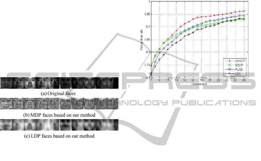
Figure 4: Training images of two subjects from the CMU
PIE database (First five columns are for one subject, last
five columns for another subject). The average Fisher ratio
of the MDP of training images by the method in (Zhang et
al., 2011) is 0.7554, while the corresponding average
Fisher ratio by our method is 0.8291.
5.1 CMU PIE Database
CMU PIE face database (Sim et al., 2003) contains
41368 face images of 68 people, each person with
13 different poses, 43 different illumination
conditions, and 4 different expressions. In our
experiments, we chose images with one near frontal
pose (C27) and all different illumination conditions
and expressions. There are 49 near frontal images
for every subject.
We chose 30 individuals from the 68 people for
our experiments. All the face images were
preprocessed with histogram equalization and
normalization. First, the images were split into two
groups. There are 25 images in group 1 for each
subject while 24 images in group 2 for each. We
randomly chose 5 images per subject from group 1
images for training, and 5 images per subject from
group 2 for testing. Figure 4 shows examples of the
original training images, the extracted MDP images
and LDP images. PCA was used to reduce the
number of dimensions of the total covariance matrix
when learning the projection
P in all the four
methods. The reported recognition rate is the
average over 50 runs.
Figure 5: Recognition rates achieved by different methods
on the CMU PIE database versus dimensionality of the
linear subspace.
Figure5 summarizes recognition performance of
various algorithms used in our experiments. From
this figure, we can see that our DSSCP algorithm
overall performs better than LDA, PLDA and SSCP.
The advantage of our algorithm becomes more
obvious at larger dimensions. This comparison
indicates image decomposition in general is
beneficial for linear subspace learning based on
LDA. Furthermore, if more discriminative
information is extracted during image decomposition
as in our algorithm, we can obtain better linear
projections during subspace learning.
5.2 Experiments on the ORL Database
ORL face database contains 400 images of 40
individuals. There are ten different images for each
subject. For some subjects, the images were taken at
different times, varying the lighting, facial
expressions (open/closed eyes, smiling/not smiling)
and facial details (glasses/no glasses). The used
ORL database is available from
http://www.zjucadcg.cn/dengcai/Data/FaceData.html.
All the images were taken against a dark
homogeneous background with the subjects in an
upright, frontal position (with tolerance for some
side movement). We selected 3 images per subject
for training, and 5 images for testing.
VISAPP2013-InternationalConferenceonComputerVisionTheoryandApplications
536
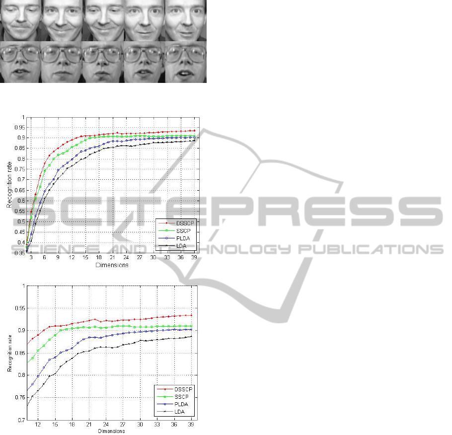
Figure 6: Face images in the ORL database.
(a)
(b)
Figure 7: Recognition rates achieved by different methods
on the ORL database vs. dimensionality of the linear
subspace. (b) shows an enlarged portion of (a).
The average recognition rates (over 50 runs) versus
subspace dimensionality are shown in Fig. 7. Fig.7
summarizes results from the algorithms tested in our
experiments. From the above figure, we can see that
DSSCP is better than LDA, PLDA and SSCP. That
means the decomposition of image is useful for
linear subspace learning based on LDA. We can
obtain a better linear subspace projection, if the
discriminative information is utilized.
6 CONCLUSIONS
In this paper, we have presented a linear subspace
learning algorithm through learning a discriminative
dictionary. Our main contributions include a new
objective function based on a Fisher ratio over
sparse coding coefficients, and its associated
algorithm for learning an overcomplete
discriminative dictionary from a set of labeled
training examples. We further obtain local MDPs
and LDPs by dividing images into rectangular
blocks, followed by blockwise feature grouping and
image decomposition. We learn a global linear
projection through the local MDPs and LDPs.
Experiments and comparisons on benchmark face
recognition datasets have demonstrated the
effectiveness of our method. Our future work
includes exploring both theoretically and empirically
the structure of the learned dictionary with respect to
different datasets and dictionary size. In addition, we
plan to investigate kernel subspace learning via
discriminative dictionaries.
REFERENCES
Belhumeur, P., Hespanha, J. and Kriengman, D. (1997).
Eigenfaces vs. Fisherfaces: Recognition using class
specific linear projection. PAMI, 19 (7): 711-720.
Boureau, Y., Bach, F., LeCun, Y., and Ponce J. (2010).
Learning Mid-level Features for Recognition. In
CVPR: 2559-2566.
Burachik, R., Kaya, C., and Mammadov, M. (2010). An
Inexact Modified Subgradient Algorithm for
Nonconvex Optimization. Computational
Optimization and Applications, 45(1): 1-24.
Cai, D., He, X., Hu, Y., Han, J., and Huang, T. (2007).
Learning a Spatially Smooth Subspace for Face
Recognition. In CVPR: 1-7.
Huang, D., Storer, M., Torre, F., and Bischof, H. (2011).
Supervised Local Subspace Learning for Continuous
Head Pose Estimation. In CVPR: 2921-2928.
Huang, K., Aviyente, S. (2007). Sparse Representation for
Signal Classification. In NIPS: 609-616.
Ji, S. Ye, J. (2008). A Unified Framework for Generalized
Linear Discriminant Analysis. In CVPR: 1-7.
Jiang, Z., Lin, Z. and Davis, L. (2011). Learning a
discriminative dictionary for sparse coding via label
consistent K-SVD. In CVPR: 1697-1704.
Kulkarni, N., Li, B. (2011). Discriminative Affine Sparse
Codes for Image Classification. In CVPR: 1609-1616.
Lee, H., Battle A., Raina, R., and Ng, A. Y. (2006).
Efficient Sparse Coding Algorithms. In NIPS: 801-
808.
Lu, J., and Tan, Y. (2010). Cost-Sensitive Subspace
Learning for Face Recognition. In CVPR: 2661-2666.
Lu, J., Plataniotis, K., Venetsanopoulos, A. (2005).
LinearSubspaceLearningbasedonaLearnedDiscriminativeDictionaryforSparseCoding
537

Regularization Studies of Linear Discriminant
Analysis in Small Sample Size Scenarios with
Application to Face Recognition. Pattern Recognition
Letters, 26(2): 181-191.
Mairal, J., Bach, F., Ponce, J. (2012). Task-Driven
Dictionary Learning. PAMI, 34(4): 791-804.
Mairal, J., Bach, F., Ponce, J., Sapiro, G. and Zisserman
A. (2008). Discriminative Learned Dictionaries for
Local Image Analysis. In CVPR: 1-8.
Neto, J., Lopes, J., Travaglia, M. (2011). Algorithms for
Quasiconvex Minimization. Optimization, 60(8-9):
1105-1117.
Qiao, Z., Zhou, L., Huang, J. Z. (2009). Sparse Linear
Discriminant Analysis with Applications to High
Dimensional Low Sample Size Data. IAENG
International Journal of Applied Mathematics, 39(1):
1-13.
Rodriguez, F., Sapiro, G. (2008). Sparse Representations
for Image Classification: Learning Discriminative and
Reconstructivenon-Parametric Dictionaries.
http://www.ima.umn.edu/preprints/jun2008/2213.pdf.
Sim, T., Baker, S., Bsat, M. (2003). The CMU Pose,
Illumination, and Expression Database. PAMI, 25(12):
1615-1618.
Turk, M., and Pentland, A. (1991). Eigenfaces for
Recognition. J. Cognitive Neuroscience, 3(1):71-86.
Yang, J., Yu, K., and Huang, T. (2010). Supervised
Translation-Invariant Sparse Coding. In CVPR: 3517-
3524.
Yang, M., Zhang, L., Feng, X., Zhang, D. (2011). Fisher
Discrimination Dictionary Learning for Sparse
Representation. In ICCV, 2011: 543-550.
Zhang, L., Zhu, P., Hu, Q., Zhang, D. (2011). A Linear
Subspace Learning Approach via Sparse Coding. In
ICCV: 755-761.
Zhang, Q., Li, B. (2010). Discriminative K-SVD for
Dictionary Learning in Face Recognition. In CVPR:
2691-2698.
Zheng, W., Lai, J., Yuen, P. (2005). GA-fisher: A New
LDA-based Face Recognition Algorithm with
Selection of Principal Components. IEEE
Transactions on Systems, Man, and Cybernetics, Part
B, 35(5): 1065-1078.
Zheng, W., Lai, J. H., Yuen, P. C., Li, S. Z. (2009).
Perturbation LDA: Learning the Difference between
the Class Empirical Mean and Its Expectation. Patten
Recognition, 42(5): 764-779.
APPENDIX
The differentiation of a sparse coefficient vector α
with respect to D is shown in (Mairal et al., 2008,
Mairal et al., 2012). Since
1
α =
TT
x
s
DD D
, where
s
in
1; 1
carries the signs of α
, its subgradient can be
computed once
α
known. It is
*
α
αα
k
jk jk
ij
ij
x
WC
D
D
, where
1
T
W
DD
,
T
CW
D
, and
α
k
denotes the k-
th nonzero component of
α
. The subgradient of an
objective function
(α )h
with respect to D is given as
follows (Mairal et al., 2012),
*
(α )(α ) α
α
TT
hh
x
DD
DD
,
where
1
( α )
=
α
T
h
DD
,
0
C
.
VISAPP2013-InternationalConferenceonComputerVisionTheoryandApplications
538
