A Neural Network and Post-processing for Estimating the Values of
Error Data
Jihoon Lee
1,2
, Yousok Kim
2
, Se-Woon Choi
1,2
and Hyo-Seon Park
1,2
1
Department of Architectural Engineering, Yonsei University, 50 Yonsei-ro, Seoul, Republic of Korea
2
Center for Structural Health Care Technology in Buildings, Yonsei University, 50 Yonsei-ro, Seoul, Republic of Korea
Keywords: Measurement Faults, Estimating Error Data, Post-processing of ANN.
Abstract: A sensor network is a key factor for successful structural health monitoring (SHM). Although stable sensor
network system is deployed in the structure for measurement, it is often inevitable to face measurement
faults. In order to secure the continuous evaluation of targeted structure in cases where the measurement
faults occur, appropriate techniques to estimate omitted or error data are necessary. In this research, back-
propagation neural network is adopted as a basic estimation method. Then, a concept of post-processing is
proposed to improve an accuracy of estimation obtained from the neural network. The results of simulation
to verify performance of estimation are also shown.
1 INTRODUCTION
A structural health monitoring (SHM) is gradually
gathering attention to guarantee safety or
serviceability in various technical fields including
civil, mechanical, and aeronautical engineering.
Most of SHMs are initiated with composition of a
sensor network designed for its purpose, and then
progress based on acquired data. Although a stable
sensor network is the primary element for further
progression of SHM process, unfortunately many
cases where acquisition of normal data is impossible
exist due to malfunction, problem in power supply,
and(or) obstacles in communication. In these cases,
normal evaluation on the status of structure, which is
an ultimate objective of SHM and sensor network,
becomes difficult until proper maintenance.
There may be two possible approaches for
continuous evaluation in case where measurement
faults occur: 1) evaluaitng a state of structure
through available data. 2) estimating the values of
unavailable data which indicates omitted or unusable
data, and then evaluating a state. This paper deals
with a proper process for estimating the values of
error data caused by measurement faults to secure
continuous SHM. A back-propagation neural
network (BPNN) which is robustly and successfully
used among various artificial neural network (ANN)
methods is adopted as a basic technique into
estimation. It allows a model-free estimation since it
only requires data for forming neural network.
Additionally, post-processing of BPNN leading to
more accurate estimation will be presented. The
post-processing is motivated from how to compose
training sets. Finally, a simulation utilizing finite
element (FE) program (OpenSees) and its results
will be discussed in regards to the performance.
2 APPLICATION OF BPNN
To achieve a final goal of this research, which is to
find an effective and model-free estimation
technique, a concrete idea is established as: to
discover the direct relationship between two types of
data sets acquired from stable sensor network in
advance to the occurrence of measurement faults.
Herein, first set is obtained from the sensors which
will face measurement faults and second set is
obtained from the sensors which will survive from
the faults. This approach enables model-free
estimation, and thus enhances applicability.
However, it is almost impossible to set the
relationship as a form of function if considering
complex systems such as building structures,
whereas ANN is most suitable for such systems.
An ANN has been widely applied on various
fields including engineering and business in order to
find the relation between inputs and outputs for the
205
Lee J., Kim Y., Choi S. and Park H..
A Neural Network and Post-processing for Estimating the Values of Error Data.
DOI: 10.5220/0004207202050208
In Proceedings of the 2nd International Conference on Sensor Networks (SENSORNETS-2013), pages 205-208
ISBN: 978-989-8565-45-7
Copyright
c
2013 SCITEPRESS (Science and Technology Publications, Lda.)

complex or ambiguous systems. BPNN utilized in
this study is based on multi-layer perceptron with
back-propagation algorithm, and is most robustly
applied among various ANN techniques. The
references for BPNN are readily available thanks to
a large number of researches on BPNN and its
applications being conducted.
Figure 1: Typical training sets for neural network.
3 TRANING SETS
3.1 Typical Training Sets
The training sets directly influence the quality of
neural network. Inputs and outputs for BPNN are
composed of measured values obtained from stable
sensor network. Figure 1 illustrates composition of
training sets which is regarded as a typical case in
this research. Inputs in typical training sets consist of
the values from active sensors that will survive after
malfunction occurrence at
*tt
and outputs consist
of the values from unstable sensors that will be
inactive due to errors in the sensors or network.
3.2 Self-referential Training Sets
Second type of training sets has different outputs
from those of typical training sets, but has identical
inputs. The outputs include input components as
shown in figure 2 and this type is named as self-
referential training sets. In case of building structure,
for example, if measurement faults occur at two
sensors among three sensors which are deployed in
close proximity, expected values of data from two
unavailable sensors can be forecasted within
acceptable range in consideration with the value
from one surviving sensor. This characteristic gives
a possibility that input components in outputs may
work as a controller to make estimated values more
acceptable.
Figure 2: Self-referential training sets.
4 A POST-PROCESSING
A neural network trained by self-referential sets
takes inputs and then reversely gives those estimated
values. Note that outputs include input components.
Nonetheless, estimated inputs and real inputs are not
identical since training of the network progresses
toward the direction of minimum error on total
estimation, but not on input components. Instead,
this point implies the opportunity to improve an
accuracy of the estimation through appropriate
adjustment processe which makes the values of
estimated and real inputs same. Thus, post-
processing of BPNN trained by self-referential sets
can be expected to improve overall accuracy of
estimation.
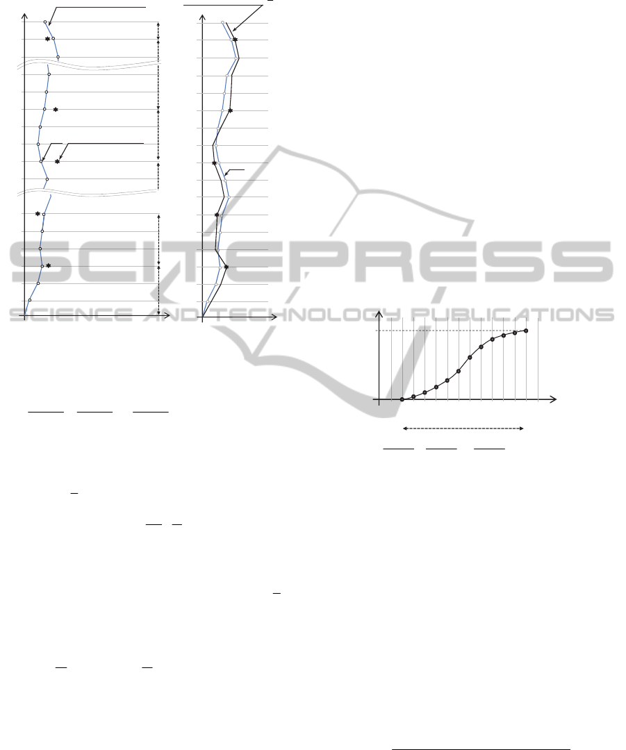
A concept of the post-processing is illustrated in
Figure 3. The post-processing is basically based on
the neural network trained by self-referential sets.
First work is numbering the outputs in accordance
with a rule that the smaller difference between data
numbers means the stronger correlation between
data. For instance, displacements of every story
show simple serial topology of correlation as shown
in Figure 3. Then, in accordance with correlation
topology, the intervals are determined by setting k
number of input components as nodes of intervals.
The key concept of post-processing is that the data
being closer to the centre of interval means the
bigger change occurs. This concept corresponds with
the expectation that extent of the correlation between
dead and surviving data will be stronger as distance
being closer each other. Regarding serial topology of
correlation, adjustment function
j
g
i
for i data in j
Data
,
Sensor 1
T
ime
t=1
Sensor 2 Sensor n
Data
,
Data
,
t=2
t=3
t=t*
Data
,
Data
,
Data
,
Data
,
Data
,
Data
,
Data
,
∗
Data
,
∗
Data
,
∗
Measurement faults
Outputs
for training
Inputs for
training
Neural
Network
estimation
Training
set 1
Training
set 2
Training
sets
Inputs for
estimation
Estimation
set 1
Inputs in a estimation set
Stable operation
Outputs in a estimation set
Outputs for
estimation
Data
,
Sensor 1
Time
Sensor 2 Sensor n
Data
,
Data
,
Data
,
Data
,
Data
,
Data
,
Data
,
Data
,
Training
set 1
Training
set 2
Measurement faults
after t=t*
Stable measurement
after t=t*
t=1
t=2
t=3
Inputs for training
(Input components in outputs)
Outputs for training
SENSORNETS2013-2ndInternationalConferenceonSensorNetworks
206

interval is derived as Equation (1) and illustrated in
Figure 4.
Figure 3: A concept of post-processing.
1
for 1 to
jj
iJ J
1
11
2
sin
2
jjj
j jj
jj jj
dJJ
g
iiJiJ
JJ JJ
(1)
with
12
0, , ,...,
k
J
II I
(2)
12
0, , ,...,
k
(3)
1
1
jj
jJ J jj
dDD
(4)
where, I is an index vector consisting of numbers of
the available data and
i
is i-th estimated value by
neural network. Finally, adjusted estimation data
i
D
in j-th interval are given by:
1
for a -th interval :
j
j
jJiJ
j
iij jJ
D
Dgi D
(5)
5 SIMULATION
To verify a performance of estimation, a simulation
was conducted. The simulation will yield two
findings: 1) accuracy of estimation by only BPNN
and 2) performance of post-processing. OpenSees,
which is FE program, and MATLAB
®
were utilized
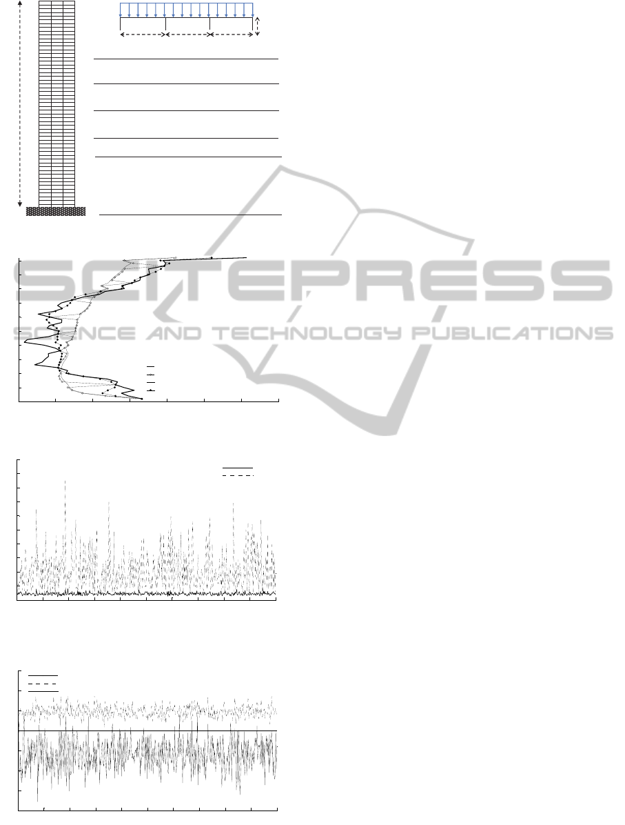
for simulation. Figure 5 displays the properties of
targeted structure. In this simulation, relative
horizontal story displacements at every story are set
as measurands. A scenario was designed as follows;
relative displacements of every story were being
stably obtained and then measurement faults
occurred at every story except 6, 12, 18, 24, 30, 36,
42, and 48 stories. In order to make a time history of
the structural response, vertical loads were
stochastically determined in each iteration according
to the uniform distribution. Thus, training sets could
be acquired by setting number of iteration as time.
This variable loads were also applied on a structure
after occurrence of measurement faults. In addition,
locations of nodes were randomly determined in
every iteration within limit range. Since real
structures show an uncertain and non-theoretical
behaviour, random dimensions were intentionally
used to reflect the uncertainty of structural behaviour.
An example of estimations is shown in Figure 6.
Figure 4: Adjustment function for serial topology of
correlation.
Figure 7 shows accuracies of 500 estimations
through BPNN trained by 200 typical sets. Root
mean square (RMS) of real displacements at every
story and root mean square error (RMSE) of
estimated displacements are used to show the
applicability of BPNN to estimation.
Meanwhile, Figure 8 expresses the performance
of post-processing compared to other cases where
the post-processing is not applied. A dashed and thin
solid lines indicate the normalized RMSE of
estimated displacements in prior to and after post-
processing, respectively. Normalized RMSE
(N.RMSE) is defined as:
befor or after post-processing
.
in case of typical training
RMSE
NRMSE
RMSE
(6)
If a value of N.RMSE after post-processing is one, it
means that the extent of reduced error is zero.
Estimation was executed for 500 times.
measured/estimated value
Output number (sensor number) (e.g. story)
1
2
3
.
.
.
.
.
.
.
.
.
1
.
.
.
.
Curve of Estimated values
through neural network trained
by self-referential set
D
j
i
D
- Measurement -
- Measurement -
1 Interval
2 Interval
Interval
1
Interval
1
.
.
.
.
.
Interval
1
Interval
Curve of adjusted values
through post-processing
- Measurement -
- Measurement -
- Measurement -
Measured values
by stable sensor network
D
measured/estimated value
D
Output number (sensor number) (e.g. story)
j
J
1j
J
O
1
11
2
() sin
2
jjj
j jj
jj jj
dJJ
g
iiJiJ
JJ JJ
interval
. . . . . . .
i
. . . . . .
ANeuralNetworkandPost-processingforEstimatingtheValuesofErrorData
207

Figure 5: The framed structure in simulation.
Figure 6: An example of estimations.
Figure 7: Accuracies of estimated displacements through
BPNN trained by 200 typical sets.
Figure 8: Performance of post-processing.
6 CONCLUSIONS
In this paper, a technique for estimating the values
of error data was dealt with in order for the stable
SHM to continue. BPNN was selected as basic tool
for model-free estimation. An efficient post-
processing of BPNN was then developed. After
neural network trained by typical sets gives first
estimated values of error data, the adjustment
process, which is a post-processing, makes those
values more accurate. Finally, the performances of
BPNN and its post-processing were verified by
conducting the FE simulation.
From the results of simulation, the estimation
through only BPNN had a stable RMSE with small
variation whatever measurand is large or not. The
presented post-processing was able to increase an
accuracy of estimation about 20% when compared
the case where BPNN is only used.
ACKONWLEDGEMENTS
This work was supported by the National Research
Foundation of Korea (NRF) grant funded by the
Korea government (MEST) (No. 2012-0001247).
REFERENCES
Heacht-Nielsen, R., 1989. Theory of the backpropagation
neural network. International Joint Conference on
Neural Network 1989. Washington, DC., Vol. 1, 593-
605.
Markos. M, Sameer. S., Novelty detection: a review-part2:
neural network based approaches, Signal Processing
83, 2499-2521.
Zhang. K., Butler. C., Yang. Q., and Lu. Y., 1996. A fibre
optic sensor for the measurement of surface roughness
and displacement using artificial neural networks.
Instrumentation and Measurement Technology
Conference 1996. Brussels, 917-920.
151m
51- story moment frame structure
20/
8m 8m
8m
3m
Information of loading and dimension
Applied probability distribution
Loading 151
Number of
variables
Parameters
Probability
property
Type of
Probability
distribution
Uniformly distribution 20±16 kN
Section (W-shape :
/
)
Beam 194×150×6/9 (ALL)
Column
396×199×7/11
(1~11F)
336×249×8/12
(12~21F)
350×175×7/11
(22~31F)
346×174×6/9
(32~41F)
250×125×6/9
(42~51F)
height of column
204 Uniformly distribution ±5mm
variable loads for every iteration (to make the training sets)
variable dimension for every iteration (to reflect the uncertainty of structure)
-8 -6 -4 -2 0 2 4 6
0
5
10
15
20
25
30
35
40
45
50
Horizontal displacement (mm)
Story
Real displacement
Estimated displacement (Typical sets)
Estimated displacement (before post-processing)
Estimated displacement (after post-processing)
0 50 100 150 200 250 300 350 400 450 500
0
2
4
6
8
10
12
14
16
18
20
Estimation number
RMS or RMSE
RMSE
RMS
0 50 100 150 200 250 300 350 400 450 500
0.2
0.4
0.6
0.8
1
1.2
1.4
1.6
Estimation number
N.RMSE
Typical training
Before post-processing
After post-processing
SENSORNETS2013-2ndInternationalConferenceonSensorNetworks
208
