
Process Monitoring in Production Systems with Large Diversity
of Products
José Gomes Requeijo
1
and Adriano Mendonça Souza
2
1
UNIDEMI, Departamento de Engenharia Mecânica e Industrial, Faculdade de Ciências e Tecnologia,
Universidade Nova de Lisboa, 2829-516 Caparica, Portugal
2
Universidade Federal de Santa Maria, Departamento de Estatística, Av. Roraima, 1000, Santa Maria, RS, Brazil
Keywords: SPC (Statistical Process Control), Control Charts, Process Capability.
Abstract: The main objectives of Statistical Process Control (SPC) are monitoring and analyzing the capability of
processes. Traditionally, the analysis of the process capability is performed at the end of Phase 1
(preliminary) and periodically during Phase 2 (monitoring) of the SPC, using the indices Cp and Cpk. SPC
and capability analysis of production systems with a large diversity of products present difficulties in
implementation. In order to meet the needs required by the current production systems, this paper presents
methods for both the statistical control and capability analysis of the processes. These methodologies
include two situations, when there are sufficient data to estimate the process parameters (mean, variance)
and when it does not exist. In the first case, it is suggested the implementation of control charts Z and W and
capability indices Z
L
and Z
U
. In the second case, when there is a limited amount of data, the authors suggest
the implementation of control charts Q and capability indices Q
L
and Q
U
. The methodologies are illustrated
with two case studies, concluding that they allow streamline the statistical control of the various processes
and reduce the downside, in Phase 2 of the SPC, where the capability analysis is made only periodically.
1 INTRODUCTION
Statistical methods play a key role in the quality
evaluation, allowing, among other things, to verify
whether the product meets the technical
specification defined. Traditionally, the most
common way of making this approach is the use of
capability indices C
p
and C
pk
. The simultaneous
analysis of these two indices allows fully evaluation
of the process’ performance, i.e., making the
comparison between the technical specifications and
tolerances of the natural process (in case the
distribution of the quality characteristic is Normally
distributed). The introduction of the C
p
index is
attributed to Juran (1974) and the introduction of the
C
pk
index is attributed to Kane (1986).
The capability analysis of processes is one of the
most effective ways to address the issue of customer
satisfaction. There are some particularly important
tasks prior to the study of C
p
and C
pk
. The control
charts are valuable tools that enable the distinction
between special causes and common causes of
variation, verification of process stability and
estimation of its parameters. Once these parameters
are estimated, we proceed to the study of process
capability.
Control charts were introduced by Shewhart
(1931), at Bell Telephone Laboratories and give a
valuable contribution to continuous quality
improvement. The control charts designed and
developed by Shewhart are typically applied to
processes that provide a large amount of data. Proper
implementation of Shewhart charts is based on the
following principles:
Samples should be homogeneous, i.e., all units are
produced under the same conditions.
The sampling frequency is defined according to
the process characteristics; so, it is expected to
maximize the opportunity of change between
samples.
The data collected should be independent, so that
the observation i of the sample j is defined by
ikik
x
(
n,,i 1
;
m,,k 1
), where
2
0
,N~
is a random variable designated by
white noise.
The data collected should follow a Normal
distribution
2
,N~X .
321
Requeijo J. and Souza A..
Process Monitoring in Production Systems with Large Diversity of Products.
DOI: 10.5220/0004203501230129
In Proceedings of the 2nd International Conference on Operations Research and Enterprise Systems (ICORES-2013), pages 123-129
ISBN: 978-989-8565-40-2
Copyright
c
2013 SCITEPRESS (Science and Technology Publications, Lda.)
The control limits of the various charts are located
to
3 standard deviations from the average
(Center Line) of the statistical distribution of the
sample in examination, corresponding to a
significance level of 0.27%.
The current situation of production systems is often
very different from that which prevailed when
Shewhart theorized statistical quality control. Today
it is necessary to consider, in the same system, the
simultaneous production of many items in smaller
amounts, which leads to the need of developing
methodologies adapted to new contexts. This issue
has been the subject of study by several researchers,
including, for example, Bothe (1988), Wheeler
(1991), Pyzdek (1993), Quesenberry (1991, 1997),
Montgomery (2012), and Pereira and Requeijo
(2012).
Thus, the statistical control of processes dealing
with various products/characteristics must be
implemented through other control charts that
provide an alternative to the Shewhart control charts.
This approach is commonly known as the statistical
control of small productions ("short runs"). The Z
and W control charts and the Q control charts are the
statistical techniques used in this context. The Z and
W charts are dimensionless and are applied when it
is possible to estimate the parameters of the different
processes. When there are insufficient data to
estimate the parameters of the processes,
Quesenberry (1991, 1997) proposes the use of
control charts Q. The implementation of these two
types of control charts (Z/W and Q) is made to take
into account - within the same document - all
products/characteristics, and provide a quick way to
easily control the stability (in-control) of all
processes.
In order to continuously evaluate the
performance of processes, these techniques present
the capability indices, Z
L
, Z
U
, Q
L
, and Q
U
introduced
by Pereira and Requeijo (2012), which enable the
analysis of the same capacity in real time.
This article discusses the two options referred,
namely, the existence or not of sufficient data to
estimate the parameters of the various processes,
considering that in both cases the study variables are
continuous, independent and normally distributed.
2 METHODOLOGY
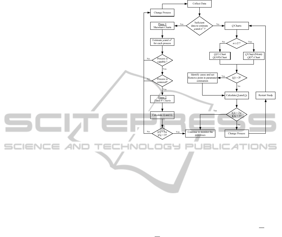
For implementation of statistical process control
when large numbers of products/characteristics are
or not available, the authors of this paper propose
the methodology described in Figure 1.
Figure 1: Methodology for Statistical Process Control with
large diversity of products.
3 SPC FOR A SIGNIFICANT
AMOUNT OF DATA
When there is sufficient data to estimate the
processes parameters, one should implement in
Phase 1 of the SPC the Shewhart control charts,
applied to each process and quality characteristic.
Usually, for continuous variables, we use the
X
and
R
,
X
and S or
X
and
M
R
control charts. Then,
in Phase 2 of the SPC, the Z and W control charts
are implemented, covering all products
/characteristics in chronological order of collection
of observations.
The analysis of the control charts help to prove
that the processes are in-control, i.e., when only
exist common causes of variation. The interpretation
of Shewhart control charts is based on the existence
of any non-random patterns (ISO 8258:1991).
3.1 Phase 1
In Phase 1, the analyst proceeds to the construction
of the most appropriate Shewhart control chart for
each product/characteristic. The upper control limit
(UCL), the lower control limit (LCL) for monitoring
these charts and the center line (CL) are determined
in Phase 1, using the formulas shown in Table 1.
ICORES2013-InternationalConferenceonOperationsResearchandEnterpriseSystems
322

Table 1: Limits of the Shewhart Control Charts (Phase 1
of SPC).
Chart LCL CL UCL
X
(Average)
SAX
RAX
3
2
or
X
SAX
RAX
3
2
or
S (Standard
Deviation)
SB
3
S
SB
4
R (Range)
RD
3
R
RD
4
MR (Moving Range)
MRD
3
M
R
MRD
4
If it is found that the process is stable
(statistically in-control) one proceeds to the
estimation of the processes parameters using
equations (1) and (2), where d
2
and c
4
are
coefficients that depend on the sample size n.
Xμ
ˆ
Xμ
ˆ
or
(1)
or or
224
d
MR
ˆ
d
R
ˆ
c
S
ˆ
(2)
The study of the capability of each process is
carried out through the classical capability indices:
6
LSLUSL
C
p
(3)
pkSpkIpk
C,CminC
(4)
3
USL
C
pkU
and
3
LSL
C
pkL
(5)
The use of equations (3) to (5) is only possible if
the quality characteristic is Normally distributed. We
suggest the use of the Kolmogorov-Smirnov test to
verify the Normality of data distribution.
If a process is not in-control the analyst should
investigate the causes that led to this situation and
make appropriate corrections. Furthtermore,
corrections should also be made in the process when
it is stable (in-control), but is not capable.
3.2 Phase 2
After stability is observed and the process capability
is analyzed in Phase 1, the statistical process control
continues through monitoring. This procedure is
commonly referred to as Phase 2 of the SPC. It
follows, in this Phase 2, the application of Z and W
control charts. These charts are built based on Z and
W statistics calculated from the sample statistics
X
(or X) and S (or R or MR), respectively. Table 2
presents the transformed Z and W statistics for the
different control charts, referring to the
product/characteristic j at time i.
The study of the performance of processes is
essential in Phase 2 of the SPC. So, it is necessary to
define the periodic analysis of the processes in this
Phase. Thus, it is suggested that this be
accomplished in real time, based on two normalized
indices (Pereira and Requeijo, 2012).
The limits for Z and W control charts are:
3
3
X
X
X
X
LCLLCL
UCLUCL
(6)
3
4
BLCL
BUCL
S
S
(7)
3
4
DLCLLCL
DUCLUCL
MRR
RR
(8)
The new normalized capability indices will be
recorded in each time r in the Z control chart. They
are defined for each j product/characteristic at
instant r by equations (9) and (10). A process of the
product/characteristic j is capable when it satisfies
simultaneously the two conditions
3
j
U
Z
and
3
j
L
Z
.
j
r
r
j
L
r
k
LSL
Z
(9)
j
r
r
j
U
r
k
USL
Z
(10)
The k value is usually 1.33 or 1.25 for bilateral
specifications or unilateral specifications,
respectively. The values
r
and
r
for the
product/characteristic j, are estimated by equations
(11) and (12) using data from the previous Phase 1
and also new data gathered during Phase 2.
Table 2: Transformed Z and W statistics.
X
Z Chart
j
X
i
j
i
XZ
X
Z
Chart
j
i
j
i
XZ
S
W
Chart
j
i
j
i
SSW
R
W
Chart
j
i
j
i
RRW
MR
W
Chart
j
i
j
i
MRMRW
ProcessMonitoringinProductionSystemswithLargeDiversityofProducts
323

XX
r
r
r
ˆ
or
ˆ
(11)
224
or or
ˆ
d
MR
d
R
c
S
rr
r
r
(12)
where:
3 2 1
1
1
,,r,XXr
r
X
rrr
(13)
3 2 1
1
1
,,r,XXr
r
X
r
rr
(14)
3 2 1
1
1
,,r,SSr
r
S
r
rr
(15)
3 2 1
1
1
,,r,RRr
r
R
r
rr
(16)
4 3 1
1
1
,,r,MRMRr
r
MR
r
rr
(17)
4 SPC FOR A LIMITED NUMBER
OF DATA
When the amount of data for each
product/characteristic is not sufficient to adequately
estimate the process parameters, it is suggested the
use of the Q statistics, which result from the
transformation of statistical sampling. Table 3
presents the Q statistics for the various charts.
The equations in Table 3 consider that
r
X
is the
observation at time r,
1r
X
is the average of
1
r
observations,
1r
S
is the standard deviation of
1
r
observations,
r
MR
is the moving range calculated at
time r,
1
is the inverse of the Normal
Distribution Function,
G
is the T-student
distribution Function with degrees of freedom,
21
,
F is the Fisher distribution Function with
1
e
2
degrees of freedom, n
i
is the size of the sample
i,
i
is the degrees of freedom of the sample i
1
ii
n
,
i
X is the average of the sample i,
i
X is
the sequencial mean of i samples,
2
i
S
is the variance
of the sample i,
2
i,p
S is the pooled variance of i
samples.
The lower and the upper control limits for the Q
control charts Q are, respectively, 3 and +3.
The processes capabilities are analyzed at every
moment through new capability indices Q
L
and Q
U
developed by Pereira and Requeijo (2012). The
estimates of these indices at time r are given by
equations (18) and (19).
Table 3: Q statistics.
XQ
Chart
4 3
1
1
1
2
1
,,r
S
XX
r
r
GXQ
r
r
r
rrr
MRQ
Chart
6 4
M
2
2
2
4
2
2
2
1
1
,,r
MRMRMR
R
FMRQ
r
r
,rr
XQ
Chart
, , i
ωGωGXQ
iiinn
i
i
ii
32
1
1
11
1
1
1
11
p,i
ii
i
ii
i
S
XX
nn
nnn
ω
i
ii
i
ii
i,p
SS
inn
SnSn
S
1 1
1
22
11
1
22
11
2
2
SQ
Chart
, , i
θFSQ
iin,nnii
ii
32
1 1
12
11
2
1
2
2
11
2
11
2
11
1 1
1
i,p
i
ii
ii
i
S
S
SnSn
Sinn
r
r
r
L
ˆ
k
ˆ
LSL
Q
ˆ
(18)
r
r
r
S
ˆ
k
ˆ
USL
Q
ˆ
(19)
XX
r
r
r
ˆ
or
ˆ
(11)
44
or cScS
ˆ
r,prr
(20)
The statistics
r
X and
r
X
are given by
equations (13) and (14). The statistic
rp
S
,
is
rnn
SnSn
S
r
ri
rp
1 1
1
22
11
,
(21)
ICORES2013-InternationalConferenceonOperationsResearchandEnterpriseSystems
324

4 3
1
1
2
2
1
2
1
,,r,XX
r
S
r
r
S
r
rrr
(22)
A process is capable if simultaneously it verifies
both conditions
3
L
Q
and
3
U
Q
.
The implementation of the Q control charts
assumes that the quality characteristic X is
independent and Normally distributed.
5 CASE STUDIES
5.1 Example 1
In this section, the authors present an example of
application to a production system of components
(connection joints) of the wiring of electrical and
electronic systems of an automotive industry. Five
products (connection joints) were selected, and the
traction resistance is the quality characteristic to be
studied.
Initially (Phase 1 of the SPC) 50 samples (each
sample was constituted by 4 connection joints) were
obtained for the five products, and the whole
procedure was as follows:
Check whether the data from each component
(connection joint) were independent, i.e.,
ijij
x
where
2
0
,N~
, by using the
Estimated Autocorrelation Function (EACF)
and the Estimated Partial Autocorrelation
Function (EPACF).
Construction of
X
and S
control charts for
each product.
Analysis of
X
and S
control charts.
Estimation of the process parameters, u X
as
the estimator of the mean and
4
cS
as the
estimator of the process standard deviation.
Check the shape of the distributions of data for
the 5 products.
Analysis of the process capability of the five
processes, using the classic capacity indices
defined by equations (3), (4) and (5).
The implementation of Phase 1 of the SPC showed
that, for all the five processes:
1)
The data for the five quality characteristics are
independent (no significant autocorrelation).
2)
The processes were in-control, i.e., there were
only common causes of variation.
3)
The data of these five distributions were
approximately Normal; this study was made
based on the Kolmogorov-Smirnov test.
4)
The five processes had the capability to
produce according to specifications.
Table 4 shows the results obtained in the study of
the processes of the 5 components (connection
joints).
After the referred study in Phase 1, the authors
moved on to Phase 2 of the SPC. As there are
several products (5 types of connection joints), the
control charts
Z
and
S
W are best fit for this
situation, since the distributions are approximately
Normal and process parameters have been estimated
in Phase 1. The authors built up the control charts
Z
and
S
W , including all components (joints) in
chronological sequence. The statistics Z and W of
the sample i for the product j were determined from
the equations of Table 2. As the technical
specification concerning the traction resistance test
of all five components is unilateral (there is only the
LSL), the authors determined only the capability
index
L
Z for each product j, at time r, calculated
using equation (9). The control charts were built
using the Excel software. Figure 2 shows these
control charts constructed from 40 samples, taken in
chronological order, referring to the five
components. The analysis of these (monitoring)
control charts reveals that the five processes are
stable, i.e., the patterns are random for each
component, and their capability to meet technical
specifications remains at a satisfactory level.
5.2 Example 2
The second example relates to the production of two
food products, which are referenced by T1 and T2.
The weight of each pack is the quality characteristic
under study. The technical specification relating to
the weight of the product packages T1 is
g 10250
and the technical specification relating to the weight
of the product packages T2 is
g 15500
.
The number of packages of each product
produced is very low. In this case, data availability
was limited to only twelve samples of T1 and ten
samples of T2. Each sample was constituted by 8
packages.
As the amount of data was restricted, this second
study applied the
XQ
and
2
SQ
control charts;
once again, Excel software was used to determine
the values of the statistics
XQ
,
2
SQ
,
L
Q and
U
Q . The resulting control charts are shown in
Figure 3.
ProcessMonitoringinProductionSystemswithLargeDiversityofProducts
325
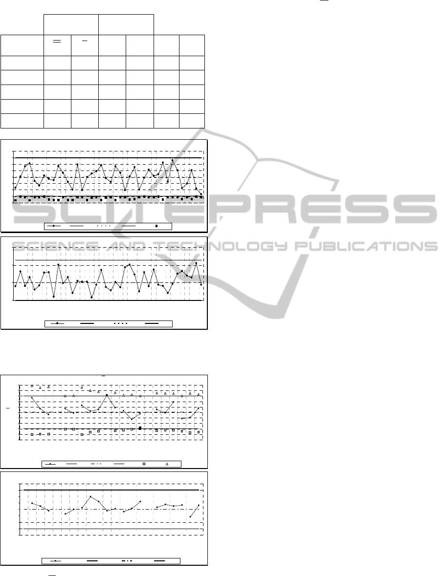
Table 4: Study of processes of five components.
Control Chart
Estimated
Parameters
Connection
Joints
X
S
ˆ
ˆ
LSL
pk
C
ˆ
U2 82.95 3.018 82.95 3.275 70 1.318
U3 113.22 2.513 113.22 2.728 100 1.615
U5 90.30 2.391 90.30 2.595 80 1.323
U7 118.91 3.232 118.91 3.508 105 1,322
U9 449.51 9.958 449.51 10.809 400 1.527
Traction Resistance -
Z
CHART
-4
-3
-2
-1
0
1
2
3
4
U9 U2 U2 U9 U2 U2 U2 U9 U9 U9 U2 U9 U9 U2 U7 U9 U7 U2 U9 U7 U2 U9 U2 U7 U9 U9 U2 U7 U5 U5 U7 U9 U7 U5 U2 U9 U2 U9 U7 U2
1 2 3 4 5 6 7 8 9 10 1112 13 14 15 16 1718 192021222324252627282930313233343536 37383940
Sa m p le
Z
Z LCL CL UCL ZL
Traction Resistance -
W
CHART
0
1
2
3
U9 U2 U2 U9 U2 U2 U2 U9 U9 U9 U2 U9 U9 U2 U7 U9 U7 U2 U9 U7 U2 U9 U2 U7 U9 U9 U2 U7 U5 U5 U7 U9 U7 U5 U2 U9 U2 U9 U7 U2
1 2 3 4 5 6 7 8 9 10 11 12 13 14 15 16 1718 192021222324252627282930313233343536 37383940
Sa m p le
W
W LCL CL UCL
Figure 2:
Z
and
S
W
Control Charts for the traction test
of 5 components (connection joints).
Q
(
X
) CHART
-5
-4
-3
-2
-1
0
1
2
3
4
5
T1 T1 T1 T1 T2 T2 T2 T1 T1 T1 T1 T1 T2 T2 T2 T2 T1 T1 T1 T2 T2 T2
1 2 3 4 5 6 7 8 9 10 11 12 13 14 15 16 17 18 19 20 21 22
Product / Sample
Q
(
X
)
Q LCL CL UCL QL QU
Q
(
S
2
) CHART
-4
-3
-2
-1
0
1
2
3
4
T1 T1 T1 T1 T2 T2 T2 T1 T1 T1 T1 T1 T2 T2 T2 T2 T1 T1 T1 T2 T2 T2
1 2 3 4 5 6 7 8 9 10 11 12 13 14 15 16 17 18 19 20 21 22
Product / Sample
Q
(
S
2
)
Q(S²) LCL CL UCL
Figure 3:
XQ e
2
SQ
Control Charts for package
weight of two products T1 and T2.
The analysis of the
XQ
control chart and
2
SQ
control chart reveals the existence of a special cause
at time t = 11 on the average of the T1 product
package. The production process is fixed up the
process and, consequently, the authors ignored the
values of the statistics at time t = 11 in the
calculation of Q statistics in the subsequent
moments. At time t = 15, it was found that the
process for product T2 showed no capability;
therefore, an intervention was made to improve the
process behavior. The study on the T2 product
process was restarted at time t = 16.
6 CONCLUSIONS
The Z and W control charts have advantages over
traditional Shewhart charts, namely:
1)
they allow statistical control of all
products/quality characteristics in the same
control chart, as well as the construction of the
X and MR control charts for each product.
2)
they allow to study different characteristics
together (i.e., simultaneously).
3)
they dramatically reduce the analysis time.
On the other hand, the possibility of making
statistical process control with a limited amount of
data is the most important advantage of the Q
control charts, solving a difficult issue in the SPC
domain. In addition to this great benefit,
implementation of Q control charts also has the
same advantages mentioned above for the Z and W
control charts.
The use of capability indices
L
Z ,
U
Z ,
L
Q and
U
Q within the Z and Q control charts allows the
study of processes capabilities in real time, thereby
decreasing the probability of producing non conform
units, i.e., it reduces the chance of producing
defective units.
In contrast with the above, a notorious
disadvantage of the Z and Q control charts is the
difficulty in analyzing the existence of non-random
patterns, increasing the complexity of this analysis
with the number of products/quality characteristics
to be checked.
REFERENCES
Bothe, D. R., 1988. SPC for Short Productions Runs,
International Quality Institute, Northville.
Juran, N. L., 1974. Juran's Quality Control Handbook,
McGraw-Hill, New York, 3
th
Edition.
ICORES2013-InternationalConferenceonOperationsResearchandEnterpriseSystems
326

Kane, V. E., 1986. Process Capability Indices, Journal of
Quality Technology
, Vol. 18, pp. 41-52.
Montgomery, D. C., 2012.
Introduction to Statistical
Quality Control
, 8
th
Edition, Wiley, New York.
Quesenberry, C. P., 1991, SPC Q Charts for Start-Up
Processes and Short or Long Runs, Journal of Quality
Technology, Vol 23, pp. 213-224.
Quesenberry, C. P., 1997. SPC Methods for Quality
Improvement, Wiley, New York.
Pereira, Z. L. and Requeijo, J. G., 2012, Qualidade:
Planeamento e Controlo Estatístico de Processos
(
Quality: Statistical Process Control and Planning),
2
nd
Edition, Foundation FCT/UNL Publisher, Lisboa.
Pyzdek, T., 1993. Process Control for Short and Small
Runs, Quality Progress, Vol. 26(4), pp. 51-60.
Shewhart, W. A., 1931.
Economic Control of Quality of
Manufactured Product
, D. Van Nostrand Company,
Inc, New York.
Wheeler, D. J., 1991. Short Run SPC, SPC Press,
Knoxville, Tennessee, 1991.
ProcessMonitoringinProductionSystemswithLargeDiversityofProducts
327
