
How to Compensate the Effect of using an Incomplete Wavelet Base
for Reconstructing an Image?
Application in Psychovisual Experiment
Sylvie Lelandais
1,2
and Justin Plantier
2
1
IBISC Laboratory, University of Evry, 40 rue du Pelvoux, 91020 Evry cedex, France
2
Department ACSO, IRBA, BP 73, 91223 Bretigny/Orge cedex, France
Keywords: Wavelet Decomposition, Psychovisual Experimentation, Difference of Gaussian Filtering.
Abstract: One way in psychovisual experiment to understand human visual system is to analyze separately contents of
different spatial frequency bands. To prepare images for this purpose, we proceed to a decomposition of the
original image by a wavelet transform centered on selected scales. The wavelets used are Difference Of
Gaussians (DOG) according to works modeling the human visual system. Before rebuilding the visual
stimulus, various transformations can be performed on different scales to measure the efficiency of the
observer, for a given task, according to the spatial frequencies used. The problem is that if we use an
incomplete wavelet basis during decomposition, there is a significant loss of information between the
original image and the reconstructed image. The work presented here offers a way to solve this problem by
using coefficients appropriate for each scale during the decomposition step.
1 INTRODUCTION
In psychovisual experiment we have to present a lot
of images to observers in order to understand how
visual human system working. The interest is to
understand which information is helpful for
performing a task as pattern recognition, distance
computation, categorization…. Objects present in
the scene are shown on different background. To
construct the psychovisual stimuli we normalize
images and we perform a wavelet decomposition of
the images to analyze, scale by scale, the observers
answer. Some experimentations have been done in
order to analyze visage perception (Gosselin, 2001)
or spatial frequencies influence on pattern
recognition capacity in complex environment
(Giraudet, 2001); (Kihara, 2010). All these
experiences and some other data obtained from
electrophysiological measures in macaque cortex
(Wilson, 1983) lead researchers to assume that it is
possible to describe the human visual system with
only a four or six frequencies channel.
The aim of this paper is to propose a method to
compensate the loss of information during image
reconstruction for a psychovisual experiment, if the
initial image decomposition has been made with few
scales, as the human visual system works.
The first part of this paper explains the choice of
Difference Of Gaussians (DOG) as wavelet
functions in the decomposition stage and the
problem when using an incomplete set of wavelets,
i.e. the loss of information problem which occurs in
the reconstruction step. We explain then the
proposal method to reduce this effect. The fourth
part is dedicated to comparative results to show how
the proposal approach reduces the explained
problem. Conclusion and some future works are
given to finish.
2 POSITION OF THE PROBLEM
Enroth-Cugell and Robson (Enroth-Cugell, 1966)
showed that the responses of the retinal ganglion
cells were type "on / off" or “off/on”, the incoming
signal on the central part being compared with the
signal arriving on the periphery of cells. This
comparison would be modeling by a DOG. Later,
models of human vision have been developed using
this type of function and applied to images, to
validate this concept (Watson, 2005). In spatial
plane (x,y), or image plane, the DOG is given by
equation (1).
271
Lelandais S. and Plantier J..
How to Compensate the Effect of using an Incomplete Wavelet Base for Reconstructing an Image? - Application in Psychovisual Experiment.
DOI: 10.5220/0004191702710275
In Proceedings of the International Conference on Bio-inspired Systems and Signal Processing (BIOSIGNALS-2013), pages 271-275
ISBN: 978-989-8565-36-5
Copyright
c
2013 SCITEPRESS (Science and Technology Publications, Lda.)
DOG
x,
y
C
e
²²
²
C
e
²²
²²
(1)
In this equation, (x,y) are the pixel coordinates in the
spatial plane, a is the scale of the DOG, C
1
=1.8 and
C
2
=0.8 in order to obtain that the Fourier transform
of the DOG is equal to zero for u=v=0 in the
frequency plane and is equal to 2.25 (Schor 1983).
The Fourier transform of a DOG is another DOG,
here called DOGTF, which is given by (2).
DOGTF
u,
v
e
²²
²
e
²²
²
(2)
In this equation, (u,v) are the frequency coordinates
and M is the number of lines (or columns) of the
image. Theoretically, when we reconstruct an image
by using its wavelets decomposition (Mallat, 1998),
final and original image would be the same. This is
partially true, if we use all the available wavelets.
Figure 1 illustrates this situation. Scale of DOG is
[0.125, 256], related to the size M of image (here we
put down M= 512). When minimum value is fixed
(SCALEINI) and total number of wavelets (NBW)
too, scale value “a” for the wavelet rank “i” is
obtained by using equation (3).
aSCALEINI2
(3)
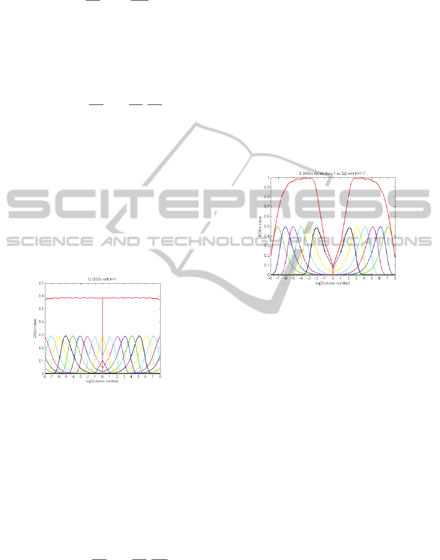
Figure 1: Twelve wavelets and their sum in red.
The DOG value (y axis) is presented related to
the binary logarithm of the vertical pixel position
(column number) as it is following defined (4).
With M2=M/2 and u=M2
if v< M2 abscissa=-log2(M2-v)
if v> M2 abscissa= log2(v-M2)
if v= M2 abscissa=-0
(4)
As you can see on figure 1, sum of all the wavelets
is not equal to one. Then, previous work (Plantier,
1992) proposes to use the equation (5) with K=1.7.
With this equation, the sum of all the wavelets is
equal to 1 on almost all space.
DOGTF
u,
v
Ke
²²
²
e
²
(5)
But if we use an incomplete set of wavelets to
reconstruct the image, there is a loss of information
for the frequencies not, or weakly, used by the
wavelets during image decomposition. These
situations are illustrated on figure 2. We use only six
DOGs with scale [1, 32]. So, in comparison with
figure 1, three wavelets are suppressed in high
frequencies (scales 0.125, 0.25 and 0.5) and three
wavelets are suppressed too in low frequencies
(scales 64, 128 and 256). Figure 2 shows the
situation, when the DOGs are computed with
equation (5) with t K=1.7, sum of wavelets is closer
to one, but only in a limited area. To conclude, if we
want to simulate an image, by using only
frequencies channel related to the human visual
system, as it is previously described with scales
[1, 32], we have to found how is it possible to
compensate this loss of information.
Figure 2: Six wavelets and their sum in red.
3 PROPOSAL METHOD
To solve this problem, we propose to make a
weighted sum of all the wavelets. So we must give a
value to each coefficient Ki as illustrated on the
equation (6).
SDOG
u,
v
K
DOGTF
u,
v
(6)
To find the value of each K
i
, we solve an equation
system with as much unknowns as wavelets we use
to decompose the image. We work on one dimension
(u=0) and we use the symmetry of the wavelets. For
each value “v” leading to a maximum value of one
of the wavelets, called “vmax
a
” with “a” the wavelet
scale, we put down the equation (7).
K
DOGTF
0,vmax
Sola
(7)
Sol(a) is the value requested for the sum of wavelets
at the position “vmax
a
”. When all the values
“vmax
a
” have been found, we have the equation
system to solve. In a first time we put down,
Sol(a)=1, a. With these solutions, sum of wavelets
BIOSIGNALS2013-InternationalConferenceonBio-inspiredSystemsandSignalProcessing
272
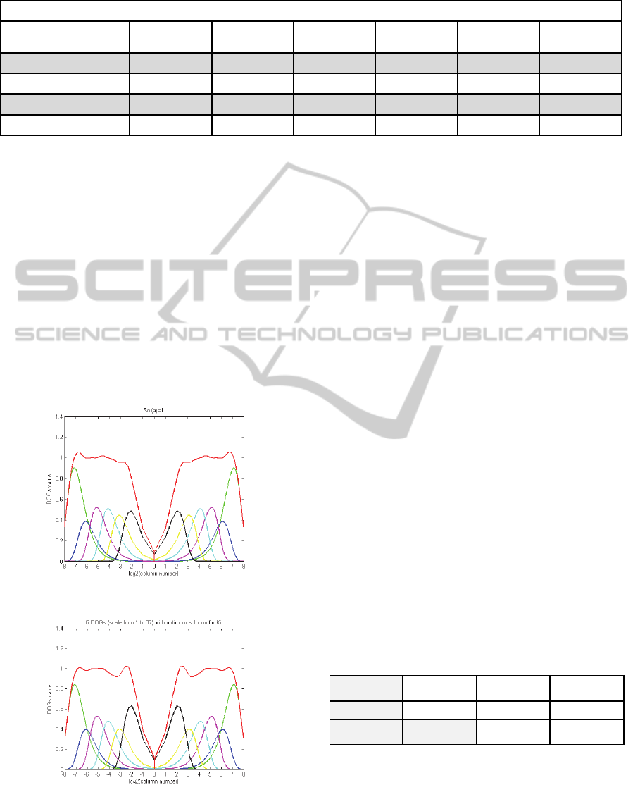
Table 1: Coefficient values obtained with Sol(a)=1, a and optimal solution.
is over “1”, for a lot of value of “v” as we can see on
figure 3. Correspondent Ki values are given in table
1. If we are over the value “1”, the reconstructed
image will be, for some frequencies different than
the original image. The goal of this work is to obtain
a reconstructed image as closer as possible to the
original image. To obtain a correct solution, we
perform an iterative resolution under two constraints
which are given by (8) and (9).
K
DOGTF
0,
v
th∀
v
(8)
1 K
DOGTF
0,
v
→0
(9)
Figure 3: Six wavelets and their sum with Sol(a)=1 a.
Figure 4: Wavelets and their sum for optimal Ki values.
So we compute 9000000 of iterations, with
different values of Sol(a) bounded by “0.8” and “1”.
The threshold th is set to 1.01. Around 85% of
possible solutions lead to a result of the equation (8)
up to the fixed threshold. To finish we obtain the Ki
coefficients given in table 1, with a gap as defined in
equation (9) equal to 0.0171. On figure 4 we show
the case for six wavelets. Sum of wavelets is more
regular and closer to “1” than in previously
solutions. A last interesting result is that Ki
coefficients obtained are almost constant for a given
number of DOGs, whatever are the size of original
image and the initial scale.
4 DISCUSSION
To evaluate the interest of these coefficients, we first
present some visual results on a natural image
(figure 5a) and its reconstructions (figure 5b and 5c).
Figure 6a and 6b display the difference between,
original and reconstructed images from figure 5. To
finish figures 6c and 6d illustrate edges detection
computed on the difference images with the Matllab
function called “Canny”. Figures 5b and 5c give a
good representation of original image with a slight
lack of contrast, as standard deviation values (STD
see table 2), illustrate it. STD is less important in
reconstructed images, and this drop is more marked
when we use the only coefficient K=1.7.
Table 2: STD and percentage of edge points in difference
images from original and reconstructed images.
The images 6a and 6b are visually close, but
when we see the edges obtained on these images, we
notice that edge points are more present in images
obtained with coefficient K=1.7 (see table 2). When
we use different coefficients K
i
in the decomposition
step, a lot of high frequencies are preserved in
Scales:
value and color
a=1
(g
reen
)
a=2
(
blue
)
a=4
(
ma
g
enta
)
a=8
(
c
y
an
)
a=16
(y
ellow
)
a=32
(
black
)
Sol(a)
1,00 1,00 1,00 1,00 1,00 1,00
Coefficient values
3,11 1,33 1,79 1,75 1,55 1,70
Sol(a)
0,95 0,97 0,99 0,97 0,90 1,00
Ki coefficients
2,94 1,31 1,79 1,74 1,25 2,25
NBW=6 - Size of image: 512x512 -SCALEINI=1
Original image
Reconstruction
with K=1,7
Reconstruction
with different Ki
STD measure 52,97 24,65 26,71
% of Edges in
Difference image
9,71% 4,13%
HowtoCompensatetheEffectofusinganIncompleteWaveletBaseforReconstructinganImage?-Applicationin
PsychovisualExperiment
273
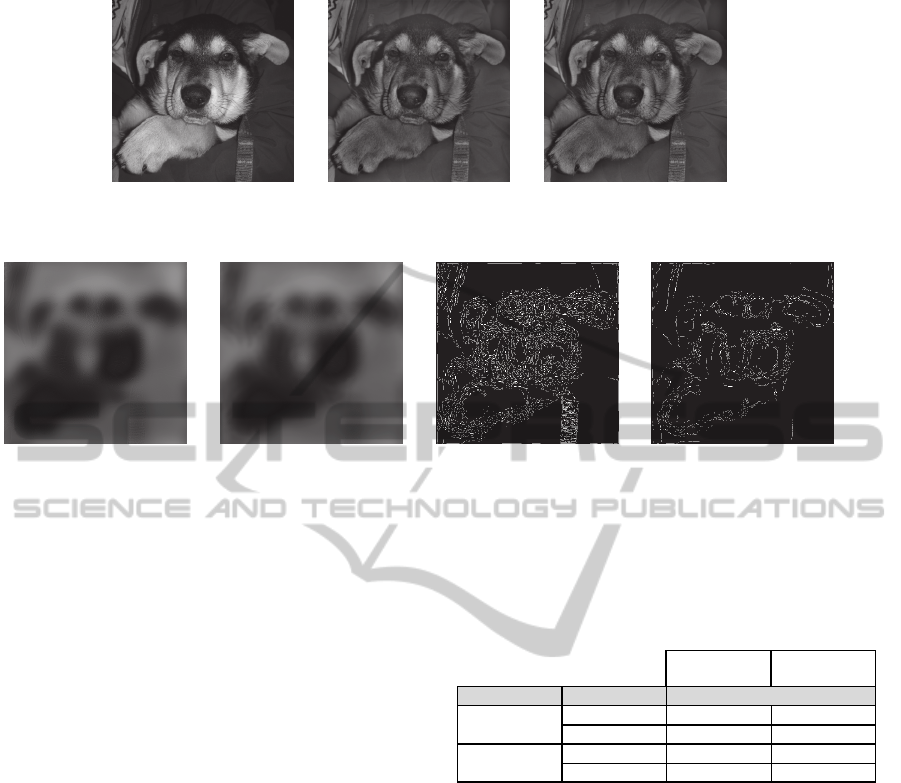
(5a) (5b) (5c)
Figure 5: 5a Original image “Ginko”, size 512x512 pixels. (5b) et (5c) reconstructed images after a decomposition by five
DOGs.(7b) by using only coefficient K=1.7 and (7c) by using proposal method.
(6a) (6b) (6c) (6d)
Figure 6a and 6b : Images of differences between 5a and 5b or 5c. Figures 6c and 6d: Edges of 6a and 6b.
reconstructed images, leading to reduce the edge
point number in the difference images.
To finish, we compared these two methods on
150 images, from the Corel Draw database. These
images are grey level converted and normalized to a
size of 512² pixels. We have chosen different kind of
images: outdoor scenes, animals, areas… Table 3
shows the results obtained by the two methods.
During the decomposition stage, five or six DOGs
have been used. As we can expect, the quality of
reconstructed images grows with the number of
wavelets used during the decomposition step. The
results confirm the interest of our approach. With the
use of Ki coefficients, we have a mean gain around
4% on the standard deviation of the reconstructed
images, and edge point number in difference images
have been divided by two, or more, when we use
five DOGs only.
5 CONCLUSIONS
This work shows the problems of image preparation
in the field of psychovisual experiment to
understand the human visual system. We could show
the problem using an incomplete wavelet basis
during the decomposition step of the image. The
proposed solution, based on assigning a special
coefficient for each scale of decomposition, has
proved effective in increasing the standard deviation
and reducing information loss for high frequencies
(edges) of the reconstructed image. Now we will use
this method in the preparation of images for
psychovisual experiments about perception and
pattern recognition in night vision images.
Table 3: Comparison of the two reconstruction methods on
150 natural images from Corel Draw Database.
REFERENCES
Enroth-Cugell C., Robson J. G., 1966. The contrast
sensitivity of retinal ganglion cells of the cat. In J.
Physiol., 187, 517-552.
Giraudet G., Roumes C. — (2001) Influence of object
background on spatial frequency processing,
Perception, 30, 26.
Gosselin F., Schyns P. G., 2001. Bubbles: a technique to
reveal the use of information in recognition tasks. In
Vision Research 41, 2261-2271.
Kihara K., Takeda Y., 2010. Time course of the
integration of spatial frequency-based information in
natural scenes. In Vision Research, 50, 2158–2162.
Mallat S., 1998. A wavelet tour of signal processing.
Academic Press.
Plantier, J. et Menu, J., 1992. Visual contrast and image
quantification from wavelet theory, In 14th Int. Conf.
of the IEEE Engineering in Medicine and Biology
Society, Paris, France.
Reconstructionwith
K=1,7
Reconstructionwith
differentKi
OriginalImages MeanofSTD
MeanofSTD 29,26 31,43
Mean%ofedge s 12,16% 4,82%
MeanofSTD 36,43 38,54
Mean%ofedge s 14,73% 7,16%
5wavelets
6wavelets
53,98
BIOSIGNALS2013-InternationalConferenceonBio-inspiredSystemsandSignalProcessing
274

Schor C. M., Wood I., 1983. Disparity range for local
stereopsis as a function of luminance spatial
frequencies. In Vision Research 23, 1649-1654.
Watson A. B., Ahumada A. J. Jr., 2005, A standard model
for foveal detection of spatial contrast. In Journal of
Vision, 5, 717–740.
Wilson, H. R., Mc Farlane, D. K., Phillips, G.C., 1983.
Spatial frequency tuning of orientation selective units
estimated by oblique maskins. In Vision Research 23,
873-882.
HowtoCompensatetheEffectofusinganIncompleteWaveletBaseforReconstructinganImage?-Applicationin
PsychovisualExperiment
275
