
Hybrid Integration of Differential Evolution with Artificial Bee Colony
for Global Optimization
Bui Ngoc Tam
1
, Pham Ngoc Hieu
1
and Hiroshi Hasegawa
2
1
Graduate School of Engineering and Science, Shibaura Institute of Technology, Saitama, Japan
2
College of Systems Engineering and Science, Shibaura Institute of Technology, Saitama, Japan
Keywords:
Artificial Bee Colony, Differential Evolution, Global Search, Hybrid Optimization Methods, Local Search,
Multi-peak Problems.
Abstract:
In this paper, we investigate the hybridization of a swarm intelligence algorithm and an evolutionary algorithm,
namely, the Artificial Bee Colony (ABC) algorithm and Differential Evolution (DE), to solve continuous
optimization problems. This Hybrid Integration of DE and ABC(HIDEABC) technique is based on integrating
the DE algorithm with the principle of ABC to improve the neighborhood search for each particle in ABC. The
swarm intelligence of the ABC algorithm and the global information obtained by the DE population approach
facilitate balanced exploration and exploitation using the HIDEABC algorithm. All algorithms were applied
to five benchmark functions and were compared using several different metrics.
1 INTRODUCTION
Two important areas of population-based optimiza-
tion algorithms are swarm intelligence (SI) algo-
rithms and evolutionary algorithms (EA). The search
strategies used by living organisms have inspired the
development of many optimization algorithms that
are currently used by numerous engineering applica-
tions. One main concept in this approach has been
to mimic how these organisms forage for food by
using search agents to find a solution to a problem.
A recent very successful algorithm in the SI class is
the artificial bee colony algorithm (ABC) (Karaboga,
2005). ABC is simple and easy to implement, but it
sometimes fails to find the global optimum in multi-
peak or high steepness problems such as the Rastri-
gin or Rosenbrock functions. ABC searches only for
the neighborhood of each employed bee or onlooker
bee in one dimension during each iteration. Thus,
the ABC algorithm component that makes employed
bees or onlooker bees move to a new food source is
too simple and this principle cannot cover the entire
search range.
Another strategy is a natural EA known as Dif-
ferential Evolution (DE), which is a population-based
parameter optimization technique that was originally
proposed by Storn and Price (Storn and Price, 1995;
Storn and Price, 1997; Price, 1999). DE is based on
the same the principle as GA where new individuals
are generated by mutation and crossover,and the vari-
ance within the population guides the choice of new
search points. DE is very powerful, but there is very
limited theoretical understanding of how it works and
why it performs well. However, DE may fall into lo-
cal optima and have a slow convergence speed during
the last stage of iterations.
To further improve the overall performance of
ABC and DE, we propose a newhybrid strategy based
on a combination of the DE and ABC algorithms. The
aim of this work is to hybridize these two successful
algorithms at a components level to benefit from their
respective strengths. Therefore, our hybrid approach
has the merits of both DE and ABC. Section 2 briefly
introduces ABC and DE. Section 3 describes HIDE-
ABC. Section 4 evaluates the performance of HIDE-
ABC using five benchmark test functions and presents
our experimental results. Our conclusions are given in
Section 5.
2 REVIEW OF STANDARD ABC
AND DE
2.1 Formulation of the Optimization
Problem
The optimization problem is formulated in this secti-
15
Ngoc Tam B., Ngoc Hieu P. and Hasegawa H..
Hybrid Integration of Differential Evolution with Artificial Bee Colony for Global Optimization.
DOI: 10.5220/0004115100150023
In Proceedings of the 4th International Joint Conference on Computational Intelligence (ECTA-2012), pages 15-23
ISBN: 978-989-8565-33-4
Copyright
c
2012 SCITEPRESS (Science and Technology Publications, Lda.)

on. The design variable, objective function, and con-
straint condition are defined as follows:
Design variable: x = [x
1
,...,x
D
] (1)
Objective function: f(x) → Minimum (2)
Constrain condition: x
lb
≤ x ≤ x
ub
(3)
where x
lb
= [x
lb
1
,...,x
lb
D
], x
ub
= [x
ub
1
,...,x
ub
D
], and D
denote the lower boundary condition vectors, upper
boundary condition vectors, and number of design
variable vectors, respectively.
2.2 Artificial Bee Colony Algorithm
(ABC)
ABC is a novel swarm intelligence (SI) algorithm,
which was inspired by the foraging behavior of hon-
eybees. ABC was first introduced by Karaboga in
2005 (Karaboga, 2005).
ABC is simple in concept, easy to implement,
and it uses few control parameters, and hence,
it has attracted the attention of researchers and
has been used widely for solving many numerical
(Karaboga and Basturk, 2007), (Karaboga and Bas-
turk, 2006) and practical engineering optimization
problems (Karaboga et al., 2007), (Baykasoglu and
Ozbakr, 2007).
There are two types of artificial bees:
- First, the employed bees that are currently exploit-
ing a food source.
- Second, the unemployed bees that are continually
looking for a food source.
Unemployed bees are divided into scout bees that
search around the nest and onlooker bees that wait at
the nest and establish communication with employee
bees.
The tasks of each type of bee are as follows:
- Employed Bee: A bee that continues to forage a
food source that it visited previously is known as an
employed bee.
- Onlooker Bee: A bee that waits in the dance area to
make a decision about a food source is known as an
onlooker bee.
- Scout Bee: When a nectar food source is abandoned
by bees, it is replaced with new a food source found
by scout bees. If a position cannot be improved fur-
ther after a predetermined number of cycles, the food
source is assumed to be abandoned. The predeter-
mined number of cycles is an important control pa-
rameter for ABC, which is known as the ”limit” be-
fore abandonment.
To better understand the basic behavioral charac-
teristics of foragers, Karaboga (Karaboga, 2005) used
figure 1. In this example, we have two discovered
Figure 1: Behavior of honeybees foraging for nectar.
food sources: A and B. At the start, a potential for-
ager is an unemployed forager. This bee will have no
knowledge of the food sources around the nest. There
are the following two possible options for this bee.
- The bee can become a scout and start searching
around the nest spontaneously for a food source ow-
ing to some internal motivation or possible external
clues (S in Figure 1).
- It can become a recruit after observing waggle
dances and start exploiting a food source (R in Fig-
ure 1).
After locating the food source, the bee memo-
rizes the location and immediately starts exploiting it.
Thus, the bee will become an employed forager. The
foraging bee collects a load of nectar from the source
and returns to the hive, before unloading the nectar in
a food store. After unloading the food, the bee has the
following three options:
- It becomes a non-committed follower after abandon-
ing the food source (UF).
- It dances and recruits nest mates before returning to
the same food source (EF1).
- It continues to forage at the food source without re-
cruiting other bees (EF2).
It is important to note that not all bees begin forag-
ing simultaneously. Experiments have confirmed that
new bees begin foraging at a rate proportional to the
difference between the eventual total number of bees
and the number that are currently foraging.
In the ABC algorithm, half of the colony consists
IJCCI2012-InternationalJointConferenceonComputationalIntelligence
16

of employed artificial bees while the other half
consists of onlookers. For every food source, there is
only one employed bee. In other words, the number
of employed bees is equal to the number of food
sources around the hive. An employed bee that
exhausts its food source becomes a scout.
ABC algorithm simulation for optimization: In
the ABC algorithm, the position of a food source i
at generation G represents a possible solution to the
optimization problem x
G
i
, while the nectar amount in
a food source corresponds to the quality (fitness fit
G
i
)
of the associated solution.
Algorithm 1: ABC Algorithm.
Requirements: Max Cycles, Colony Size, Limit.
Begin
1: Initialize the food sources
x
G=0
i, j
= lb
j
+ rand
j
∗(ub
j
−lb
j
) (4)
where rand
j
a random number in [0,1].
2: Evaluate the food sources
3: Cycle = 1
4: while (Cycle ≤ Max
cycle) do
5: Produce new solutions using employed bees
v
i, j
= x
i, j
+ ϕ
i, j
∗(x
i, j
−x
k, j
) (5)
where k ∈ {1, 2, .., SN} and j ∈ { 1,2,..,D} are ran-
domly selected indices. Although k is determined ran-
domly, it has to be different from i. ϕ
ij
is a random
number between [−1, 1]. v
i, j
is the neighborhood of
x
i, j
in dimension j.
6: Evaluate the new solutions and apply a greedy se-
lection process
7: Calculate the probability values using the fitness
values
p
i
=
fit
G
i
SN
∑
n=1
fit
G
n
(6)
where fit
G
i
is the fitness of food source i at generation
G.
8: Produce new solutions using onlooker bees
v
i, j
= x
i, j
+ ϕ
i, j
∗(x
i, j
−x
k, j
) (7)
9: Apply a greedy selection process for onlooker bees
10: Determine the abandoned solutions and generate
new solutions randomly using scouts
x
G=0
ij
= lb
j
+ rand
j
∗(ub
j
−lb
j
) (8)
where rand
j
a random number in [0,1].
11: Memorize the best solution found so far
12: Cycle = Cycle + 1
13: end while
14: return best solution
End
2.3 Differential Evolution (DE)
Algorithm
DE was proposed by Storn and Price (Storn and Price,
1995) and is a very popular EA, which delivers re-
markable performance with a wide variety of prob-
lems from diverse fields. Like other EAs, DE is a
population-based stochastic search technique. It uses
mutation, crossover, and selection operators at each
generation to move its population toward the global
optimum.
The DE technique combines simple arithmetic op-
erators with the classical methods of crossover, muta-
tion, and selection to evolve from a randomly gener-
ated starting population to a final solution.
At each generation G, DE creates a mutant vector
v
G
i
= (v
G
i,1
,v
G
i,2
,...,v
G
i,D
) for each individual x
G
i
(known
as a target vector) in the current population. The five
widely used DE mutation scheme operators are as fol-
lows (Wang, 2011).
DE/rand/1 scheme:
v
G+1
i, j
= x
G
r
1
, j
+ F(x
G
r
2
, j
−x
G
r
3
, j
) (9)
DE /best /1 scheme:
v
G+1
i, j
= x
G
best, j
+ F(x
G
r
1
, j
−x
G
r
2
, j
) (10)
DE/target-to-best/1 scheme:
v
G+1
i, j
= x
G
i, j
+ F((x
G
best, j
−x
G
i, j
) + (x
G
r
1
, j
−x
G
r
2
, j
)) (11)
DE/best/2 scheme:
v
G+1
i, j
= x
G
best, j
+ F((x
G
r
1
, j
−x
G
r
2
, j
) + (x
G
r
3
, j
−x
G
r
4
, j
))
(12)
DE/rand/2 scheme:
v
G+1
i, j
= x
G
r
1
, j
+ F((x
G
r
2
, j
−x
G
r
3
, j
) + (x
G
r
4
, j
−x
G
r
5
, j
)) (13)
In the above equations, r
1
, r
2
, r
3
, r
4
, and r
5
are distinct
integers, which have been selected randomly from the
range [1, 2,...,NP] and they are also different from i.
The parameter F is called the scaling factor, which
amplifies the difference vectors. x
G
best
is the best indi-
vidual in the current population.
After mutation, DE performs a binomial crossover
operator on x
G
i
and v
G
i
to generate a trial vector
u
G
i
= (u
G
i,1
,u
G
i,2
,...,u
G
i,D
)
u
G
i, j
=
(
v
G
i, j
if rand
j
(0,1) ≤CR or j = j
rand
x
G
i, j
otherwise
(14)
where i = 1, 2,...,NP, j = 1,2,...,D, j
rand
is a ran-
domly chosen integer from [1,D], rand
j
(0, 1) is a
uniformly distributed random number between 0 and
1 that is generated for each j, and CR ∈ [0,1] is the
crossover control parameter. Because of the use of
HybridIntegrationofDifferentialEvolutionwithArtificialBeeColonyforGlobalOptimization
17
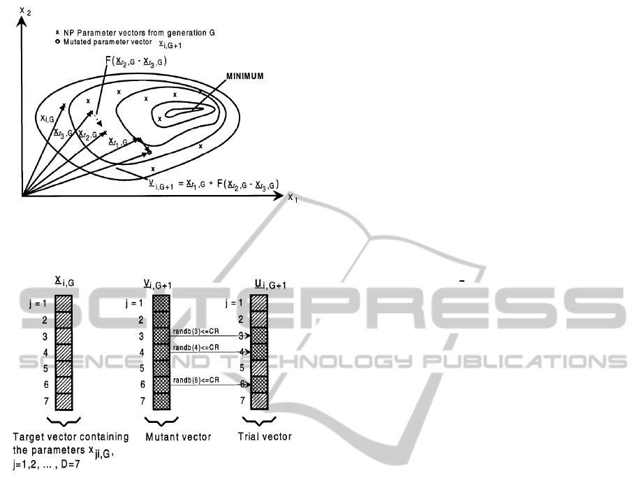
Figure 2: Example of a two-dimensional cost function
showing its contour lines and the process of generating mu-
tations of DE/rand/1.
Figure 3: Illustration of the crossover process with D = 7.
j
rand
, the trial vector u
G
i
differs from its target vector
x
G
i
.
A selection operation is performed to choose whether
the target vector x
G
i
or the trial vector u
G
i
should enter
the next generation.
x
G+1
i
=
(
u
G
i
if f(u
G
i
) ≤ f(x
G
i
)
x
G
i
otherwise
(15)
The DE control parameters comprise the population
size NP, the scaling factor F, and the crossover
control parameter CR. Storn and Price (Storn and
Price, 1995) argued that it is not difficult to set these
three control parameters to obtain good performance.
They suggested that NP should lie between 5D and
10D; a good initial choice for F is 0.5, whereas a
value of F lower than 0.4 or higher than 1.0 will lead
to performance degradation, and CR can be set to 0.1
or 0.9.
(Ronkkonen et al., 2005) suggested that NP
should lie between 2D and 4D; F should be selected
from the range [0.4, 0.95], with F = 0.9 being
a good trade-off between convergence speed and
robustness; and CR should lie between 0.0 and 0.2
for separable functions, and between 0.9 and 1.0 for
multimodal and non-separable functions. Clearly,
these researchers agreed that F should be in the range
of [0.4, 1.0], and that CR should be close to 1.0 or
0.0, depending on the characteristics of problems.
Algorithm 2: DE Algorithm.
Requirements: Max Cycles, number of particles NP,
crossover constant CR, and scaling factor F.
Begin
1: Initialize the population
x
G=0
ij
= lb
j
+ rand
j
∗(ub
j
−lb
j
) (16)
where rand
j
a random number in [0,1].
2: Evaluate the population
3: Cycle = 1
4: while (Cycle ≤Max
cycle) for each individual x
G
i
do
5: Mutation: DE creates a mutation vector v
G
i
us-
ing equations (9) to (13), depending on the mutation
scheme
6: Crossover: DE creates a trial vector u
G
i
using equa-
tion (14)
7: Greedy selection: To decide whether it should be-
come a member of generation G + 1 (next generation),
the trial vector u
G
i
is compared to the target vector x
G
i
(15)
8: Memorize the best solution found thus far
9: Cycle = Cycle+ 1
10: end while
11: return best solution
End
3 HYBRID INTEGRATED DE AND
ABC ALGORITHM (HIDEABC)
(Talbi, 2002) presented several hybridization methods
for heuristic algorithms. According to (Talbi, 2002),
two algorithms can be hybridized at a high level or
low level using relay or co-evolutionary methods,
which may be homogeneous or heterogeneous.
In this study, we hybridized ABC with DE
using a low-level co-evolutionary heterogeneous
hybrid approach. The hybrid is low-level because
we combined the functionality of both algorithms.
It is co-evolutionary because we did not use both
algorithms in series, i.e., they run in parallel. Finally,
it is heterogeneous because two different algorithms
are used to produce the final results.
DE has many advantages, but it still has scope
for improvement. In our test, we readily found that
the DE did not always reach the best solution for a
problem, because the algorithm sometimes reached
IJCCI2012-InternationalJointConferenceonComputationalIntelligence
18

a local optimum. To solve this problem, we propose
a hybrid DE based on the ABC algorithm. In our
proposed hybrid, we use the crossover and mutation
principles of EA to enhance the neighborhood search
of ABC.
The major difference between DE and ABC
is how new individuals are generated. The new
individuals generated during each generation are
known as offsprings. The basic idea of HIDEABC
is to combine the SI capacity of ABC with the local
search capability of DE. In order to combine these
algorithms, HIDEABC is proposed as follows. To
generate new individuals in ABC, we use equations
(9) to (13), depending on the mutation scheme, while
equation (18) is used for DE crossover to enhance the
neighborhood search of employed bees and onlooker
bees.
The main steps of the HIDEABC algorithm are as fol-
low:
• Step 1: In the first step, HIDEABC generates a
randomly distributed initial population P(G = 0)
of SN solutions (food source positions), where SN
denotes the size of the food source. Each so-
lution (food source) x
i
(i = 1,2, ..., SN) is a D-
dimensional vector, where D is the number of op-
timization parameters.
• Step 2: Send the employed bee to the food sources
and calculate their nectar amounts, before a new
food source is found.
In this process, the modification strategy uses the
classical mutation and crossover components of
the DE algorithm. This operation also improves
the convergence speed and increases the diver-
sity of the ABC population. We use equations (9)
to (13), depending on the mutation method, with
eq(14) for crossover.
• Step 3: An onlooker bee chooses a food source
depending on the probability value associated
with that food source, p
i
: equation (7)
• Step 4: Send the onlooker bees to the food
sources and determine their nectar amounts. Each
onlooker evaluates the nectar information from all
employed bees and selects a food source depend-
ing on the nectar amount available at the sources.
The employed bee modifies the source position in
her memory and checks its nectar amount. Pro-
vided that the nectar level is higher than that of
the previous level, the bee memorizes the new po-
sition and forgets the old position.
Use equations (9) to (13), depending on the muta-
tion method with equation (14) for crossover.
• Step 5: A food source that is abandoned by bees
is replaced with a new food source by the scouts.
If a position cannot be improved further during a
predetermined number of cycles limit, then that
food source is assumed to be abandoned.
• Step 6: Send the scouts to the search area ran-
domly to discover new food sources using equa-
tion (17).
• Step 7: Memorize the best food source found so
far in the global best memory.
• Repeat: Steps 2 to 7 until the terminal require-
ments are met.
Algorithm 3: HIDEABC Algorithm.
Requirements: Max Cycles, number of particles NP,
limit, crossover constant CR, and scaling factor F.
Begin
1: Initialize the food source positions
x
G=0
ij
= lb
j
+ rand
j
∗(ub
j
−lb
j
) (17)
where rand
j
is a random number in [0,1].
2: Evaluate the food sources
3: Cycle = 1
4: while (Cycle ≤ Max
cycle) do
5: Produce new solutions using employed bees
Mutation process: Use equations (9) to (13), depend-
ing on the mutation scheme, to generate v
G
i
Crossover process:
u
G
i, j
=
v
G
i, j
if rand
j
(0,1) ≤CR or j = j
rand
x
G
i, j
otherwise
x
G
i, j
+ ϕ
i, j
∗(x
G
i, j
−x
G
k, j
) if j = para2change
(18)
where i = 1,2,...,NP, j = 1,2,...,D, j
rand
and
para2change are randomly chosen integers from
[1,D], rand
j
(0, 1) is a uniformly distributed random
number between 0 and 1 generated for each j, and
CR ∈ [0, 1] is the crossover control parameter. Be-
cause of the use of j
rand
, the trial vector u
G
i
differs
from its target vector x
G
i
, and k ∈ {1,2,..,SN} is a
randomly chosen index [1,NP]. Although k is deter-
mined randomly, it should be different from i. ϕ
ij
is a
random number between [-1,1].
6: Evaluate the new solutions and apply a greedy se-
lection process using equation (15).
7: Calculate the probability values based on their fit-
ness values using equation (9).
8: Produce new solutions using onlooker bees; the
process of neighborhood search by onlooker bees is
the same as that used by employed bees.
9: Apply a greedy selection process to onlooker bees
using equation (15).
10: Determine the abandoned solutions and generate
new solutions randomly using scouts using equation
HybridIntegrationofDifferentialEvolutionwithArtificialBeeColonyforGlobalOptimization
19

(11).
11: Memorize the best solution found so far
12: Cycle = Cycle + 1
13: end while
14: return the best solution
End
4 EXPERIMENTS
The first experiment tuned the F and CR parameters
for DE and HIDEABC. Next, the F and CR parame-
ters produced by the first test were used to compare
the robustness of the optimization approach. These
experiments involved 50 trials for each function. The
initial seed number was varied randomly during each
trial.
4.1 Benchmark Functions
To estimate the stability and convergence to the op-
timal solution using HIDEABC, we used five bench-
mark functions with 20 dimensions, namely, Rastri-
gin (RA), Ridge (RI), Griewank (GR), Ackley (AC),
and Rosenbrock (RO). These functions are given as
follows.
RA : f
1
= 10n+
n
∑
i=1
{x
2
i
−10cos(2πx
i
)} (19)
RI : f
2
=
n
∑
i=1
i
∑
j=1
x
j
!
2
(20)
GR : f
3
= 1+
n
∑
i=1
x
2
i
4000
−
n
∏
i=1
cos
x
i
√
i
(21)
AC : f
4
= −20exp
−0.2
s
1
n
n
∑
i=1
x
2
i
!
−exp
1
n
n
∑
i=1
cos(2πx
i
)
!
+ 20 + e(22)
RO : f
5
=
n
∑
i=1
[100(x
i+1
−x
2
i
)
2
+ (x
i
−1)
2
] (23)
For each function, Table 1 lists the characteris-
tics including the dependent terms, multi-peaks, and
steepness. All of the functions are minimized to zero
when the optimal variables x
opt
= 0 and RO function
x
opt
= 1 are obtained. Note that it is difficult to search
for optimal solutions by applying a single optimiza-
tion strategy, because each function has specific com-
plex characteristics.
Table 2 summarizes the design range variables.
The search process is terminated when the search
point reaches an optimal solution or a current genera-
tion process reaches the termination point.
Table 1: Characteristics of the benchmark functions.
Function Dependent Multi-peaks Steepness
RA No Yes Average
RI Yes No Average
GR Yes Yes Small
AC No Yes Average
RO Yes No High
Table 2: Design range variables of the benchmark functions.
Function Design range
RA −5.12 ≤x ≤5.12
RI −51.2 ≤x ≤51.2
GR −51.2 ≤x ≤51.2
AC −5.12 ≤ x ≤ 5.12
RO −2.048 ≤ x ≤ 2.048
4.2 Tuning of F and CR Parameters for
DE and HIDEABC
As mentioned above, the DE control parameters such
as the population size NP, scaling factor F, and
crossover control parameter CR are highly sensitive.
In this test, we determined the best values of F and
CR for each function using each approach. We tested
50 runs each for DE and HIDEABC. The population
size was NP = 8D = 160, F = 0.05, 0.1,...,0.95,1.0,
CR = 0.05,0.1,...,0.95, 1.0, and Max
cycle = 2500.
The experiment results are summarized in Table 3.
The solutions of all benchmark functions reached
their global optimum solutions.
4.3 Testing the Robustness of the
Algorithms
4.3.1 Setting the Parameters for Standard ABC
The population size was NP = 160. The onlooker
bees and employed bees constituted 50% each of the
colony population, SN = NP/2 = 80, FoodNumber=
80, and Limit = FoodNumber∗D.
4.3.2 Setting the Parameters for DE and
HIDEABC
The population size was NP = 160. The F and CR
values in Table 3 were used in the test, with the
IJCCI2012-InternationalJointConferenceonComputationalIntelligence
20
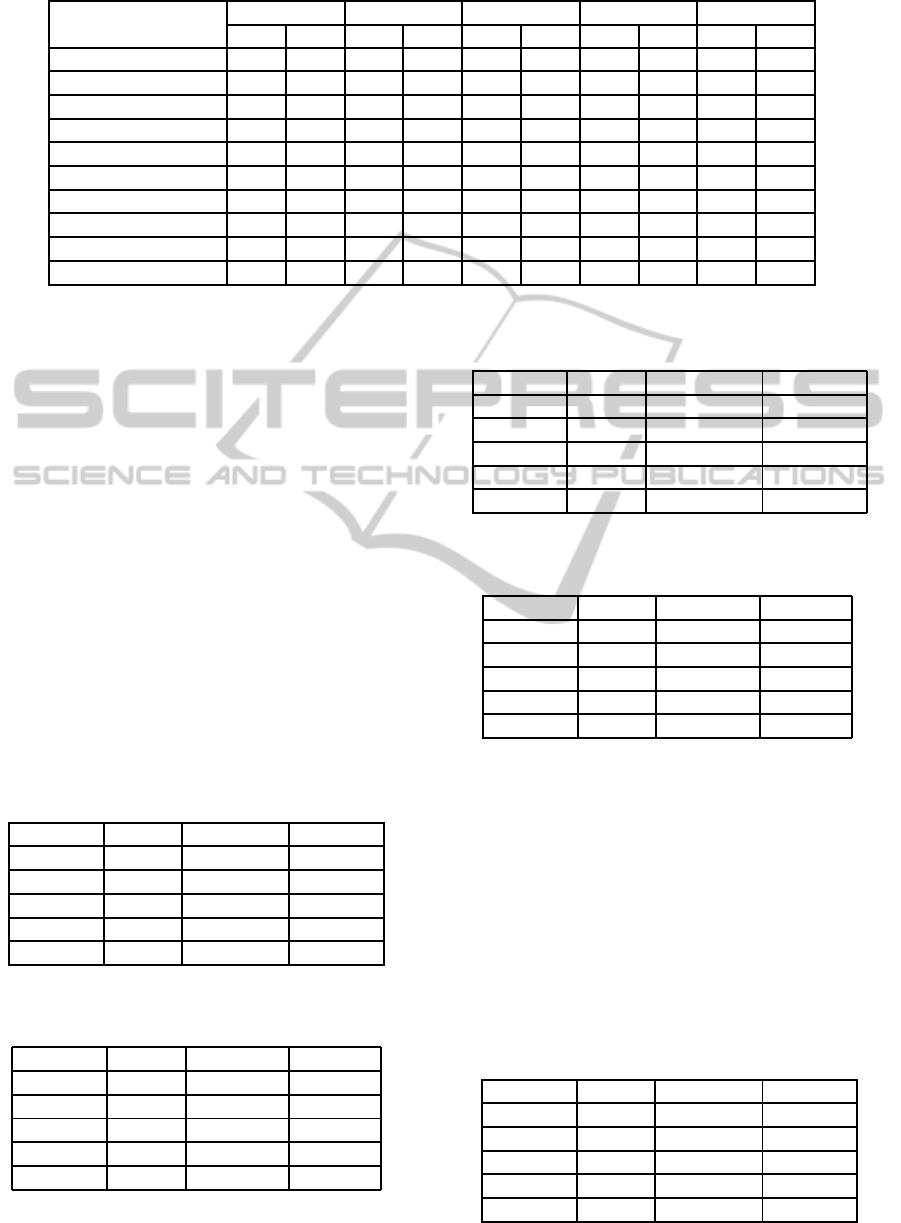
Table 3: Best values for F and CR using 20 dimensions.
Function
RA RI GR AC RO
F CR F CR F CR F CR F CR
DE/rand/1 0.10 0.15 0.55 0.95 0.15 0.65 0.15 0.65 0.45 0.95
DE/best/1 0.50 0.05 0.75 0.95 0.50 0.65 0.40 0.40 0.70 0.70
DE/target/1 0.50 0.05 0.65 0.95 0.55 0.85 0.45 0.50 0.65 0.65
DE/best/2 0.30 0.05 0.55 1.00 0.35 0.65 0.35 0.50 0.50 0.80
DE/rand/2 0.05 0.10 0.35 1.00 0.10 0.65 0.10 0.55 0.35 0.95
HIDEABC/rand/1 0.50 0.05 0.35 0.90 0.25 0.90 0.40 0.35 0.75 0.75
HIDEABC/best/1 0.50 0.05 0.35 0.90 0.30 0.90 0.50 0.50 0.65 0.65
HIDEABC/target/1 0.95 0.05 0.65 0.90 0.50 0.80 0.50 0.75 0.60 0.65
HIDEABC/best/2 0.50 0.05 0.65 1.00 0.20 0.90 0.35 0.55 0.55 0.75
HIDEABC/rand/2 0.10 0.10 0.50 1.00 0.15 0.60 0.15 0.55 0.40 0.95
same accuracy (eps = 1.0e
−6
) to compare the iter-
ation when the optimum was satisfied. If the suc-
cess rate of the optimal solution was not 100%, ”–”
is shown in Tables 4 to 8. We refer to HIDEABC/...
as H/... for convenience.
Tables 4 to 8 show that the hybrid HIDEABC
reached the global optimum in fewer iterations than
with ABC and DE for all functions, with the excep-
tion of the RI function. The hybrid method failed to
achieve better results with the RI function.
Tables 3 and 8 show that the results with HIDE-
ABC/rand were good for the RA function, while Ta-
bles 7 and 8 show that they were good for the RI
function. Tables 5, 6, and 7 show that the results
were good with GR, that the AC function was good
with HIDEABC/target/1, and that the RO function
was good with HIDEABC/best/1. This problem de-
pended on the function’s characteristics (see Table 1)
and the control parameters F and CR.
Table 4: Number of iterations required to reach global opti-
mum (Average results for 50 trials).
Function ABC DE/rand/1 H/rand/1
RA 543.10 349.62 253.10
RI – 1670.80 1079.00
GR 246.84 106.26 12.63
AC 571.60 224.98 78.60
RO – 1328.02 712.72
Table 5: Number of iterations required to reach global opti-
mum (Average results for 50 trials).
Function ABC DE/best/1 H/best/1
RA 543.10 451.88 311.50
RI – 815.98 1102.20
GR 246.84 55.56 12.90
AC 571.60 281.74 79.80
RO – 1237.54 592.69
Table 6: Number of iterations required to reach global opti-
mum (Average results for 50 trials).
Function ABC DE/target/1 H/target/1
RA 543.10 716.36 398.43
RI – 581.68 1118.07
GR 246.84 59.34 31.33
AC 571.60 170.0 73.00
RO – 1196.98 539.52
Table 7: Number of iterations required to reach global opti-
mum (Average results for 50 trials).
Function ABC DE/best/2 H/best/2
RA 543.10 574.62 407.03
RI – 546.94 841.30
GR 246.84 55.28 12.23
AC 571.60 148.46 73.13
RO – 1049.56 957.50
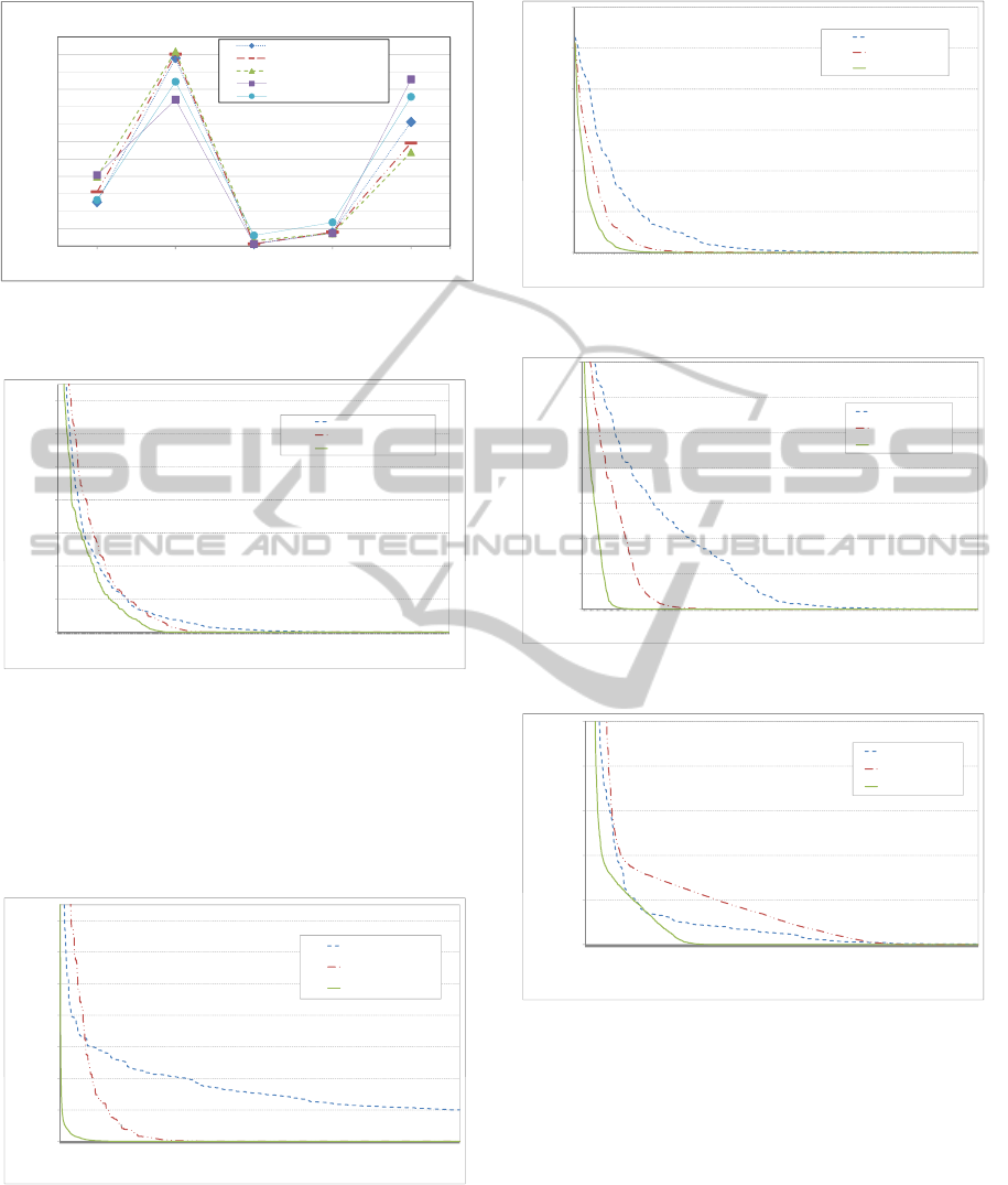
Figures 5 to 9 show the average fitness of in-
dividual solutions until these methods reached the
global optimum solutions. Numerical experiments
showed that HIDEABC improved the generation
number compared with the average generation results
using simple ABC and DE. All benchmark functions
reached their global optimum solutions. However,
there were some differences among the methods.
HIDEABC converged faster than ABC and DE, and
it was particularly effective for the RO function.
Table 8: Number of iterations required to reach global opti-
mum (Average results for 50 trials).
Function ABC DE/rand/2 H/rand/2
RA 543.10 329.72 265.50
RI – 469.26 944.37
GR 246.84 104.52 60.83
AC 571.60 235.50 135.70
RO – 1336.84 856.80
HybridIntegrationofDifferentialEvolutionwithArtificialBeeColonyforGlobalOptimization
21
0
100
200
300
400
500
600
700
800
900
1000
1100
1200
Rastrigin
Ridge
Griewank
Ackley
Rosenbrock
iteration
Number of iterations are required to reach the global
optimum, eps=1E-6
HIDEABC_rand/1
HIDEABC_best/1
HIDEABC_target/to/best/1
HIDEABC_best/2
HIDEABC_rand/2
Figure 4: Number of iterations required to reach the global
optimum using HIDEABC.
6.00E+01
8.00E+01
1.00E+02
1.20E+02
1.40E+02
fitness value
function f0(Rastrigin)
ABC
DE/rand/1
HIDEABC_rand/1
0.00E+00
2.00E+01
4.00E+01
6.00E+01
8.00E+01
1.00E+02
1.20E+02
1.40E+02
1
13
25
37
49
61
73
85
97
109
121
133
145
157
169
181
193
205
217
229
241
253
265
277
289
301
313
325
337
349
361
373
385
397
409
421
433
445
457
469
481
493
505
517
529
541
553
565
577
589
fitness value
iteration
function f0(Rastrigin)
ABC
DE/rand/1
HIDEABC_rand/1
Figure 5: Convergence graph for the Rastrigin function.
HIDEABC arrived at the global optimum with a
high probability for every function. In summary, this
validation confirmed that the HIDEABC strategy
can reduce the computational costs and improve the
stability during convergence to the optimal solution.
4.00E+03
6.00E+03
8.00E+03
1.00E+04
1.20E+04
1.40E+04
fitness value
function f1( Ridge)
ABC
DE/rand/1
HIDEABC_rand/1
0.00E+00
2.00E+03
4.00E+03
6.00E+03
8.00E+03
1.00E+04
1.20E+04
1.40E+04
1
30
59
88
117
146
175
204
233
262
291
320
349
378
407
436
465
494
523
552
581
610
639
668
697
726
755
784
813
842
871
900
929
958
987
1016
1045
1074
1103
1132
1161
1190
1219
1248
1277
1306
1335
1364
1393
1422
1451
1480
fitness value
iteration
function f1( Ridge)
ABC
DE/rand/1
HIDEABC_rand/1
Figure 6: Convergence graph for the Ridge function.
1.00E+00
1.50E+00
2.00E+00
2.50E+00
3.00E+00
fitness value
function f2 (Griewank)
ABC
DE/rand/1
HIDEABC_rand/1
0.00E+00
5.00E-01
1.00E+00
1.50E+00
2.00E+00
2.50E+00
3.00E+00
1
4
7
10
13
16
19
22
25
28
31
34
37
40
43
46
49
52
55
58
61
64
67
70
73
76
79
82
85
88
91
94
97
100
103
106
109
112
115
118
121
124
127
130
133
136
139
142
145
148
fitness value
iteration
function f2 (Griewank)
ABC
DE/rand/1
HIDEABC_rand/1
Figure 7: Convergence graph for the Griewank function.
2.00E+00
3.00E+00
4.00E+00
5.00E+00
6.00E+00
7.00E+00
fitness value
function f3( Ackley)
ABC
DE/rand/1
HIDEABC_rand/1
0.00E+00
1.00E+00
2.00E+00
3.00E+00
4.00E+00
5.00E+00
6.00E+00
7.00E+00
1
7
13
19
25
31
37
43
49
55
61
67
73
79
85
91
97
103
109
115
121
127
133
139
145
151
157
163
169
175
181
187
193
199
205
211
217
223
229
235
241
247
253
259
265
271
277
283
289
295
fitness value
iteration
function f3( Ackley)
ABC
DE/rand/1
HIDEABC_rand/1
Figure 8: Convergence graph for the Ackley function.
2.00E+01
3.00E+01
4.00E+01
5.00E+01
fitness value
function f4(Rosenbrock)
ABC
DE/rand/1
HIDEABC_rand/1
0.00E+00
1.00E+01
2.00E+01
3.00E+01
4.00E+01
5.00E+01
1
43
85
127
169
211
253
295
337
379
421
463
505
547
589
631
673
715
757
799
841
883
925
967
1009
1051
1093
1135
1177
1219
1261
1303
1345
1387
1429
1471
fitness value
iteration
function f4(Rosenbrock)
ABC
DE/rand/1
HIDEABC_rand/1
Figure 9: Convergence graph for the Rosenbrock function.
5 CONCLUSIONS
This paper introduces a new hybrid algorithm that ex-
ploits the strengths of ABC and DE. Our main con-
cept is to integrate the exploitation capacities of ABC
with the exploration abilities of DE. Five benchmark
functions were used to validate the performance of
HIDEABC compared with standard ABC and DE.
The results showed that HIDEABC outperformed
both tests for most functions. The results demon-
strated that the convergence speed was faster with
IJCCI2012-InternationalJointConferenceonComputationalIntelligence
22

HIDEABC than with ABC and DE.
In this study, we separated the F and CR parame-
ters for each function in each method, and hence we
had to tune these parameters. In future work, we will
try to develop adaptive or self-adaptive F and CR.
We confirmed that HIDEABC reduced the calculation
costs and improved the time required for convergence
to the optimal solution.
REFERENCES
Baykasoglu, A. and Ozbakr, L. (2007). Artificial bee colony
algorithm and its application to generalized assign-
ment problem, swarm intelligence: Focus on ant and
particle swarm optimization. In I-Tech Education and
Publishing, Vienna, Austria.
Karaboga, D. (2005). An idea based on honey bee
swarm for numerical optimization. In TECHNICAL
REPORT-TR06.
Karaboga, D., Akay, B., and Ozturk, C. (2007). Artificial
bee colony (abc) optimization algorithm for training
feed-forward neural networks. In Modeling Decisions
for Artificial Intelligence.
Karaboga, D. and Basturk, B. (2006). An artificial bee
colony (abc) algorithm for numeric function optimiza-
tion. In IEEE Swarm Intelligence Symposium 2006,
Indianapolis, Indiana, USA.
Karaboga, D. and Basturk, B. (2007). A powerful and
efficient algorithm for numerical function optimiza-
tion:artificial bee colony (abc) algorithm. In Journal
of Global Optimization.
Price, K. (1999). An introduction to differential evolution.
In Corne, D., Dorigo, M., Glover, F. (eds.) New Ideas
in Optimization.
Ronkkonen, J., Kukkonen, S., and Price, K. (2005). Real
parameter optimization with differential evolution. In
IEEE CEC, vol. 1.
Storn, R. and Price, K. (1995). Differential evolution: A
simple and efficient adaptive scheme for global op-
timization over continuous spaces. In Comput. Sci.
Inst., Berkeley, CA, Tech. Rep. TR-95-012.
Storn, R. and Price, K. (1997). Differential evolution a sim-
ple and efficient heuristic for global optimization over
continuous spaces. In Journal of Global Optimization.
Talbi, E. G. (2002). A taxonomy of hybrid metaheuristic.
In Journal of Heuristics.
Wang, Y. (2011). Differential evolution with composite trial
vector generation strategies and control parameters. In
IEEE Transactions on Evolutionary Computation.
HybridIntegrationofDifferentialEvolutionwithArtificialBeeColonyforGlobalOptimization
23
