On the Capacity of Hopfield Neural Networks as EDAs for Solving
Combinatorial Optimisation Problems
Kevin Swingler
Computing Science and Maths, University of Stirling, Stirling, FK9 4LA, Scotland, U.K.
Keywords:
Optimisation, Hopfield Neural Networks, Estimation of Distribution Algorithms.
Abstract:
Multi-modal optimisation problems are characterised by the presence of either local sub-optimal points or a
number of equally optimal points. These local optima can be considered as point attractors for hill climbing
search algorithms. It is desirable to be able to model them either to avoid mistaking a local optimum for
a global one or to allow the discovery of multiple equally optimal solutions. Hopfield neural networks are
capable of modelling a number of patterns as point attractors which are learned from known patterns. This
paper shows how a Hopfield network can model a number of point attractors based on non-optimal samples
from an objective function. The resulting network is shown to be able to model and generate a number of local
optimal solutions up to a certain capacity. This capacity, and a method for extending it is studied.
1 INTRODUCTION
Optimisation based on an objective function (OF) in-
volves finding an input to the OF that maximises its
output
1
. In many cases the OF has a structure that can
be exploited to speed a search considerably. There
are many algorithms that guide a search by sampling
from an objective function. Estimation of Distribution
Algorithms (EDAs) (M
¨
uhlenbein and Paaß, 1996),
(Shakya et al., 2012) build a model of the probability
of sub-patterns appearing in a good solution, and then
generate new solutions by sampling based on those
probabilities. Objective function models (Jin, 2005)
estimate the OF by fitting a model to selected samples
and then search the model. Population based meth-
ods such as Genetic Algorithms (Goldberg, 1989),
(De Jong, 2006) and Particle Swarm Optimisation
(Kennedy, 2001) do not build an explicit model, but
maintain a population of high scoring points to guide
the sampling of new points.
Any OF of interest is likely to be multi-modal,
which means that it contains more than one local
maxima. An algorithm that guides the sampling of
the OF towards high points is likely to reach a lo-
cal maximum before it finds the global maximum.
A local maximum is a point which has no immedi-
ate neighbours in input space with a higher output. If
we assume that the OF surface is smooth (or can be
smoothed) then each local maximum sits at the top of
1
Optimisation might alternatively minimise a cost func-
tion, but in this paper we maximise.
a hill delimited on all sides by local minima. A hill
climb from any point on the slopes of this hill will
take you to the local maximum so local maxima can
be considered as attractor states for a hill climbing al-
gorithm. One way to manage the problem of local
maxima is to model these attractor states. This paper
shows how a neural network can be used to explicitly
model the attractor states of an OF and investigates
the number of attractors a model can carry.
The motivation for using a Hopfield network is
that it can model multiple point attractors in high di-
mensional space. The dynamics of such networks
means they are guaranteed to move from any point
in input space to a point of local maximum. Hopfield
networks have been thoroughly studied so if they are
capable of modelling the attractors of an OF, then this
large body of existing research may be immediately
applied. In this paper we present evidence that Hop-
field networks can learn the attractor states of arbi-
trary OFs from a relatively small number of function
samples.
Paper Structure. This paper first describes the con-
cepts of objective functions and attractors in objec-
tive function space. Section 2 describes the standard
Hopfield neural network and section 3 introduces the
Hopfield EDA (HEDA) and addresses its capacity to
store local maxima as attractor states. Sections 4 and
5 describe how to train and search a HEDA using two
different learning algorithms. Section 6 shows the re-
sults of some experiments investigating the capacity
of different HEDA models and section 7 offers some
conclusions and future directions.
152
Swingler K..
On the Capacity of Hopfield Neural Networks as EDAs for Solving Combinatorial Optimisation Problems.
DOI: 10.5220/0004113901520157
In Proceedings of the 4th International Joint Conference on Computational Intelligence (ECTA-2012), pages 152-157
ISBN: 978-989-8565-33-4
Copyright
c
 2012 SCITEPRESS (Science and Technology Publications, Lda.)

1.1 The Problem Space
We consider binary patterns over c where:
c = c
1
,...,c
n
c
i
∈ {−1,1} (1)
We denote the objective function as:
f (c) = x x ∈R (2)
Local maxima in f (c) can be viewed as the peaks
of hills with monotonically increasing slopes. Each
of these hills is an attractor in the search space and a
simple hill climbing search from any point on its slope
will lead to the hill’s attractor point. The goal is to find
one or more patterns in c that maximise f (c) and to
avoid local maxima. We will do this by modelling the
attractor states.
2 HOPFIELD NETWORKS
Hopfield networks (Hopfield, 1982) are able to store
patterns as point attractors in n dimensional binary
space. Traditionally, known patterns are loaded di-
rectly into the network (see the learning rule 5 below),
but in this paper we investigate the use of a Hopfield
network to discover point attractors by sampling from
an objective function. A Hopfield network is a neural
network consisting of n simple connected processing
units. The values the units take are represented by a
vector, u:
u = u
1
,...,u
n
u
i
∈ {−1,1} (3)
The processing units are connected by symmetric
weighted connections:
W = [w
i j
] (4)
where w
i j
is the strength of the connection from unit
i to unit j. Units are not connected to themselves,
i.e. w
ii
= 0 and connections are symmetrical, i.e.
w
i j
= w
ji
. The values of the weighted connections
define the point attractors and learning in a standard
Hopfield network takes place by setting the pattern to
be learned using formula 6 and applying the Hebbian
weight update rule:
w
i j
 w
i j
+ u
i
u
j
∀i 6= j (5)
A single pattern, c is set by
∀i u
i
 c
i
(6)
where  indicates assignment. Pattern recall is per-
formed by allowing the network to settle to an attrac-
tor state determined by the values of its weights. The
unit update rule during settling is
a
i

∑
w
ji
u
j
(7)
where a
i
is a temporary activation value, following
which the unit’s value is capped by a threshold, θ,
such that:
u
i


1 if a
i
> θ
−1 otherwise
(8)
In this paper, we will always use θ = 0. The pro-
cess of settling repeatedly uses the unit update rule of
formulae 7 and 8 for a randomly selected unit in the
network until no update produces a change in unit val-
ues. At that point, the network is said to have settled.
The symmetrical weights and zero self-connections
mean that the network is a Lyapunov function, which
guarantees that the network will settle to a fixed point
from any starting point.
With the above restrictions in place, the network
has an energy function that determines the set of pos-
sible stable states into which it will settle. The energy
function is defined as:
E = −
1
2
∑
i, j
w
i j
u
i
u
j
(9)
Settling the network, by formulae 7 and 8 pro-
duces a pattern corresponding to a local minimum of
E in equation 9. Hopfield networks have been used to
solve optimization tasks such as the travelling sales-
man problem (Hopfield and Tank, 1985) but weights
are set by an analysis of the problem rather than by
learning. In the next section, we show how random
patterns and an objective function can be used to train
a Hopfield network as a search technique.
3 HOPFIELD EDAS
We define a Hopfield EDA (HEDA) as an EDA imple-
mented by means of a Hopfield neural network. Al-
though a traditional Hopfield network contains only
second order connections, we will allow higher order
networks and denote a HEDA of order m by HEDA
m
.
We will concentrate mostly on second order models
based on the traditional Hopfield network - HEDA
2
models.
3.1 HEDA Capacity
The capacity of a HEDA is the number of distinct at-
tractors it can model. As each attractor is a single lo-
cal maximum, the capacity of the network determines
the number of local maxima a HEDA can absorb on
its way to the global maximum.
OntheCapacityofHopfieldNeuralNetworksasEDAsforSolvingCombinatorialOptimisationProblems
153

There is a limit on the number of attractor states
a Hopfield network can represent. For random pat-
terns, (McEliece et al., 1987) states that the capacity
of such a network is n/(4 ln n) where n is the number
of elements in the model.
(Storkey and Valabregue, 1999) suggest an alter-
native to the Hebbian learning rule that increases the
capacity of a Hopfield network. This new learning
rule can be used to increase the number of attractors
in a HEDA
2
and so increase the number of local max-
ima it is able to model. A Hopfield network of order
2 trained with Storkey’s learning rule has a capacity
of n/
√
2lnn.
The Hopfield approach described for HEDA
m
can
be extended to higher orders, with a corresponding
increase in storage capacity, along with an associ-
ated exponential increase in processing time. (Kub-
ota, 2007) states that the capacity of order m associa-
tive memories is O(n
m
/lnn).
4 TRAINING A HEDA
In this section we describe a method for training a
HEDA
2
. The principles apply equally to HEDAs of
higher order. During learning, candidate solutions are
generated randomly one at a time. Each candidate so-
lution is evaluated using the objective function and the
result is used as a learning rate in the Hebbian weight
update rule (see update rule 10). Consequently, each
pattern is learned with a different strength, which re-
flects its quality as a solution.
4.1 The New Weight Update Rule
Hopfield networks have a limited capacity for storing
patterns. If a number of patterns greater than this ca-
pacity are learned, patterns interfere with each other
producing spurious states, which are a combination of
more than one pattern. To learn the point attractors of
local optima without ever sampling those points, we
need to create spurious states that are a combination
of lower points. We do this by over-filling a Hop-
field network with samples and introducing a strength
of learning so that higher scoring patterns contribute
more to the new spurious states. This yields a simple
modification to the Hebbian rule:
w
i j
 w
i j
+ f (c)u
i
u
j
(10)
where f (c) is the objective function. This has the
effect of learning high scoring second order sub-
patterns more than lower scoring ones. Note that due
to the symmetry of the weight connections, each at-
tractor has an associated inverse pattern that is also an
attractor. The means that both the pattern and its in-
verse may need to be scored to tell the solutions apart
from their inverse twins.
4.2 The Learning Algorithm
The learning algorithm proceeds as follows:
1. Set up a Hopfield network with W
i j
=0 for all i, j
2. Repeat the following until one or more stopping
criteria are met
(a) Generate a random pattern, c, where each c
i
has
an equal probability of being set to 1 or -1
(b) Calculate f (c) by equation 2
(c) Load c using formula 6
(d) Update the weight matrix W using the learning
rule in formula 10
Stop when a pattern of required quality has been
found or when the attractor states become stable or
the network reaches capacity.
5 SEARCHING A HEDA MODEL
Once a number of solutions have been found, the net-
work will have a number of local attractors. By pre-
senting a new pattern and allowing the network to set-
tle, the closest solution (or locally optimal solution)
will be found. This settling does not require f (c) to be
evaluated. In cases where a partial solution is already
known, the HEDA may be used to find the closest lo-
cal optimum. Where the global optimum is required,
the model needs to be searched. This is quite fast be-
cause the objective function does not have to be eval-
uated very often. The search could be carried out in
a random fashion, picking points and settling to their
attractor states until an acceptable score is produced,
or using a more sophisticated search method such as
simulated annealing (Hertz et al., 1991).
5.1 Improving Capacity
Storkey (Storkey and Valabregue, 1999) introduced
a new learning rule for Hopfield networks that in-
creased the capacity of a network compared to using
the Hebbian rule. The new weight update rule is:
w
i j
 w
t−1
i j
+
1
n
u
i
u
j
−
1
n
u
i
h
ji
−
1
n
u
j
h
i j
(11)
where
h
i j

∑
k6=i, j
w
t−1
ik
u
k
(12)
IJCCI2012-InternationalJointConferenceonComputationalIntelligence
154

and w
t−1
i j
is the weight at the previous time step.
The new terms, h
ji
and h
i j
have the effect of cre-
ating a local field around w
i j
that reduces the lower
order noise brought about by the interaction of differ-
ent attractors.
To use this learning rule in a HEDA, we make the
following alterations to the update rules:
w
i j
 w
t−1
i j
+
1
n
(u
i
u
j
−u
i
h
ji
−u
j
h
i j
) f (p) (13)
and
h
i j

∑
k6=i, j
w
t−1
ik
u
k
β (14)
where β < 1 is a discount parameter that controls how
much damping is applied to the learning rule.
6 EXPERIMENTAL RESULTS
The following experimental results test the new learn-
ing rules. We first introduce the objective functions
used and then describe the experiments.
6.1 Experimental Objective Functions
We use two types of objective function: a set of dis-
tinct target patterns and a concept that contains depen-
dencies of order 2.
In the first case, the set of target patterns are de-
noted as the set t:
t = {t
1
,...,t
s
} (15)
We then define the objective function as an inverse
normalised weighted Hamming distance between c
and each target pattern t
j
in t as.
f (c|t
j
) = 1 −
∑
δ
c
i
,t
ji
n
(16)
where t
ji
is element i of target j and δ
c
j
,t
ji
is the Kro-
necker delta function between pattern element i in t
j
and its equivalent in c. We take the score of a single
pattern to be the maximal score of all the members of
the target set.
f (c|t) = max
j=1...s
( f (c|t
j
)) (17)
6.2 Testing HEDA
2
Capacity by
Learning and Searching
This set of experiments compares the capacity of a
normally trained Hopfield network with the search ca-
pacity of a HEDA
2
. We will compare two learning
rules (Hebbian and Storkey). The experiments are re-
peated many times, all using randomly generated tar-
get patterns where each element has an equal proba-
bility of being +1 or -1.
6.2.1 Experiment 1 - Hebbian HEDA
2
Capacity
In experiment 1 we compare Hebbian trained Hop-
field networks with their equivalent HEDA
2
models.
The aim is to discover whether or not the HEDA
2
model can obtain the capacity of the Hopfield net-
work. Hopfield networks were trained on patterns us-
ing standard Hebbian learning, with one pattern at a
time being added until the network’s capacity was ex-
ceeded. At this point, the learned patterns were set to
be the targets for the HEDA
2
search and the network’s
weights reset.
100 repeated trials were made training HEDA
2
networks ranging in size from 10 to 100 units in steps
of 5. For each trial, the capacity of the trained net-
work, the number of those patterns discovered by ran-
dom sampling and the time taken to find them all was
recorded.
Results. Regardless of the capacity or size of the
Hopfield network, the HEDA
2
search was always able
to discover every pattern learned during the capacity
filling stage of the test. From this, we can conclude
that the capacity of a HEDA
2
for storing local optima
is the same as the capacity for the equivalent Hopfield
network when searching for a set of random targets.
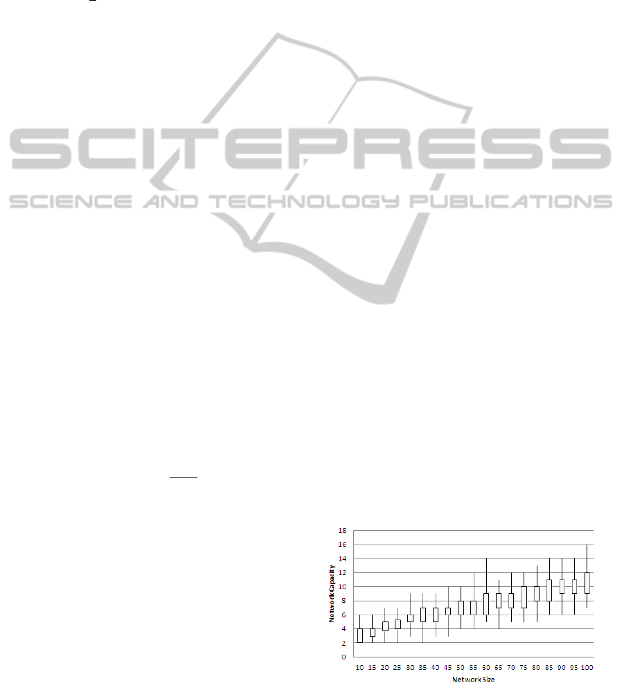
Figure 1 shows the relationship between Hopfield
network size and capacity. The spread of capacity val-
ues is wide - varying with the level of interdependence
between the random patterns. The chart shows the
range and the inter-quartile range of capacity for each
network size.
Capacity is linear with network size in terms of
units, but the number of weights in a network in-
creases quadratically with capacity.
Figure 1: The learned capacity of HEDA
2
models of various
sizes across 100 trials.
OntheCapacityofHopfieldNeuralNetworksasEDAsforSolvingCombinatorialOptimisationProblems
155

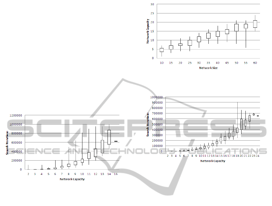
Figure 2 shows the number of samples required to
find all patterns against network capacity. By curve
fitting to the data shown, we find that the number of
samples required to find all solutions is quadratic with
number of solutions.
In fact, as the search space grows, the number
of iterations required to fully characterise the search
space, as a proportion of the size of search space di-
minishes exponentially. For networks of size 100, the
search space has 2
100
possible states and the HEDA
2
is able to find all of the targets in an average of
around 355,000 samples. That is a sample consisting
of 2.8
−25
of all possible patterns. In this modelling
exercise, no evolution towards a target took place; the
learning took place using random sampling.
Figure 2: The number of trials needed to find all local op-
tima in a Hopfield network filled to capacity, plotted against
the number of patterns to find.
6.2.2 Experiment 2 - Storkey HEDA
2
Capacity
In experiment 2 we repeat experiment 1 but use the
Storkey learning rule rather than the Hebbian version.
The experimental procedure is the same as that de-
scribed above, except that we only have samples from
networks up to size 60, as the process for larger net-
works is very slow.
Results. As with the Hebbian learning, Storkey
trained HEDA
2
search was always able to discover
every pattern learned during the capacity filling stage
of the test. This shows that the improved learning rule
will deliver the increased capacity for capturing local
optima that we sought. The cost of this capacity is a
far slower learning algorithm, however.
Figure 3 shows the relationship between Hopfield
network size and capacity for the Storkey trained net-
work.
Figure 4 shows the number of samples required
to find all patterns against network size when using
the Storkey rule. Again, we see that search iterations
increase quadratically with network capacity.
Figure 3: The learned capacity of Storkey trained HEDA
2
models.
Figure 4: The number of trials needed to find all local
optima in a Hopfield network filled to capacity using the
Storkey learning rule, plotted against the number of patterns
to find.
6.3 Experiments with Second Order
Patterns
The concept of vertical symmetry in a pattern involves
a second order rule. It is not possible to score the con-
tribution of pattern elements in isolation - each one
must be considered with its mirror partner. By design-
ing an objective function that scores a pattern in terms
of its symmetry, we show how a HEDA
2
can learn a
second order concept and so generate many patterns
that score perfectly against this concept, despite hav-
ing never seen any such patterns during training.
Patterns were generated in a 6 x 6 image of bi-
nary pixels. There are 2
36
(68,719,476,736) possible
patterns in such a matrix. Of those, there will be one
vertically symmetrical pattern for every possible pat-
tern in one half of the image. There are 2
18
(262,144)
such half patterns, representing 0.00038% of the total
number of possible patterns.
In this trial the network was allowed to learn un-
til ten different symmetrical patterns had been found.
At this point, the learning process was terminated and
the network was tested with a set of local searches de-
signed to count the number of attractor states learned.
IJCCI2012-InternationalJointConferenceonComputationalIntelligence
156

Results. Across 50 trials, the 36 node HEDA took
an average of 9932 pattern evaluations before it ter-
minated having found 10 perfect scoring patterns.
A record of the samples made showed that none of
the randomly generated patterns used during train-
ing gained a perfect score, so the network was only
trained on less than perfect patterns. The average
trained model’s capacity was found to be 132, which
gives an average of 75 OF evaluations per pattern
found. Figure 5 shows two examples of random start-
ing patterns and their associated attractor states.
Figure 5: Two examples of fixed point attractors of the
HEDA
2
trained on the second order concept of symmetry.
The left hand column shows random starting points and the
right hand column shows the associated point attractor state.
7 CONCLUSIONS
It is possible to adapt both the Hebbian and Storkey
learning rules for Hopfield networks to allow them to
learn the attractor states corresponding to multiple lo-
cal maxima based on random samples from an objec-
tive function. We have experimentally shown that the
capacity of these networks is at least equal to the ca-
pacity of a Hopfield network trained directly on the
attractor points.
Networks trained in this way are able to find a set
of attractors by undirected sampling - that is with no
evolution of solutions - in a number of samples that is
a very small fraction of the size of the search space.
In a second order network, as network size, n
varies, we have seen that search space grows expo-
nentially with n, the number of local optima that can
be stored grows linearly with n and the time to find all
local optima grows quadratically with n.
Future work will address a number of area includ-
ing higher order networks and networks of variable
order; an evolutionary approach to training the net-
works when the number of local optima is higher than
the capacity of the network; the effects of spurious at-
tractors; the use of the Energy function of equation 9
as a proxy for objective function evaluations; and the
smoothing of noisy landscapes. Hopfield networks
have been extensively studied so there is a wealth of
research on which to draw during future work.
ACKNOWLEDGEMENTS
Thank you David Cairns and Leslie Smith for your
helpful comments on earlier versions of this paper.
REFERENCES
De Jong, K. (2006). Evolutionary computation : a unified
approach. MIT Press, Cambridge, Mass.
Goldberg, D. E. (1989). Genetic Algorithms in Search, Op-
timization, and Machine Learning. Addison-Wesley
Professional, 1 edition.
Hertz, J., Krogh, A., and Palmer, R. G. (1991). Introduc-
tion to the Theory of Neural Computation. Addison-
Wesley, New York.
Hopfield, J. J. (1982). Neural networks and physical sys-
tems with emergent collective computational abili-
ties. Proceedings of the National Academy of Sciences
USA, 79(8):2554–2558.
Hopfield, J. J. and Tank, D. W. (1985). Neural computa-
tion of decisions in optimization problems. Biological
Cybernetics, 52:141–152.
Jin, Y. (2005). A comprehensive survey of fitness approxi-
mation in evolutionary computation. Soft Computing
- A Fusion of Foundations, Methodologies and Appli-
cations, 9:3–12.
Kennedy, J. (2001). Swarm intelligence. Morgan Kaufmann
Publishers, San Francisco.
Kubota, T. (2007). A higher order associative memory with
mcculloch-pitts neurons and plastic synapses. In Neu-
ral Networks, 2007. IJCNN 2007. International Joint
Conference on, pages 1982 –1989.
McEliece, R., Posner, E., Rodemich, E., and Venkatesh,
S. (1987). The capacity of the hopfield associative
memory. Information Theory, IEEE Transactions on,
33(4):461 – 482.
M
¨
uhlenbein, H. and Paaß, G. (1996). From recombination
of genes to the estimation of distributions i. binary pa-
rameters. In Voigt, H.-M., Ebeling, W., Rechenberg,
I., and Schwefel, H.-P., editors, Parallel Problem Solv-
ing from Nature PPSN IV, volume 1141 of Lecture
Notes in Computer Science, pages 178–187. Springer
Berlin / Heidelberg.
Shakya, S., McCall, J., Brownlee, A., and Owusu, G.
(2012). Deum - distribution estimation using markov
networks. In Shakya, S. and Santana, R., editors,
Markov Networks in Evolutionary Computation, vol-
ume 14 of Adaptation, Learning, and Optimization,
pages 55–71. Springer Berlin Heidelberg.
Storkey, A. J. and Valabregue, R. (1999). The basins of at-
traction of a new hopfield learning rule. Neural Netw.,
12(6):869–876.
OntheCapacityofHopfieldNeuralNetworksasEDAsforSolvingCombinatorialOptimisationProblems
157