
A Non-lineal Mathematical Model for Annealing Stainless Steel Coils
Raquel González Corral, J. Bonelo Sánchez
Acerinox Europa S.A., Fabrica Campo de Gibraltar 11370 Los Barrios, Cadiz, Spain
Carlos G. Spinola, C. Galvez-Fernández, M. Martín-Vázquez
Dept of Electronics, University of Malaga, TCC S.L., Robinson Crusoe 5, 29006 Malaga, Spain
Keywords: Annealing, Self Organizing Map, Temperature, Heat, Stainless Steel, Furnace.
Abstract: Stainless steel manufacturing has experienced a high growth. Nowadays the stainless steel manufacturing is
an industry with many applications. Annealing process is an important process in the production of stainless
steel coils. The aim of this research is to obtain the classification of defective annealed coils. So a nonlinear
mathematical model has been developed for the annealing process. In this research the following techniques
have been used: SOM neural networks and classifications methods. For testing, temperature signals were
collected along the annealing furnace, also speed signal of the production line were collected. These signals
are correlated with each one of the manufactured coils.
1 INTRODUCTION
The conventional method to model the heating of a
furnace consist on solving simultaneously the
equations for radiation, convection and transmission.
This study proposes a new approach, using data
mining tools and neural networks to schedule and
control the annealing furnace line for stainless steel.
The following data are available: speed, temperature
and the parameters of the furnace. With these data
annealed coils can be classified in well annealed
coils and bad annealed coils. The following aims are
pursued: Reducing energy consumption, optimizing
output temperature, improving the surface quality
and optimizing the annealing time to increase
productivity.
2 ANNEALING PROCESS
The purpose of the annealing process is to remove
metal defects, to make it easier to work with. In cold
rolling, the thickness of a coil is reduced to the
desired thickness, but this process gives raise to
deformation in the crystalline structure of the metal,
that can be recovered by annealing. The annealing is
usually associated with other complementary
processes, such as superficial pickling. Resulting in
a production line type AP (Annealing and Pickling).
A coil circulates inside the annealing furnace
whose temperature must be maintained during the
time required on order that the annealing process to
occur. This time depends on the material thickness,
ranging from one to five minutes. The furnace is
divided into six zones, each one of which has its
burners and temperature control. The calculation of
temperature points determine the ideal amount of
heat to be transferred to the zone controllers,
according to optimum heat-up curve (Spinola,
2008).
Figure 1: Annealing furnace.
3 AIMS
The target of the investigation is to individually
analyze annealing of each coil, considering the
607
González Corral R., Bonelo Sánchez J., G. Spinola C., Galvez-Fernández C. and Martín-Vázquez M..
A Non-lineal Mathematical Model for Annealing Stainless Steel Coils.
DOI: 10.5220/0004112206070610
In Proceedings of the 4th International Joint Conference on Computational Intelligence (NCTA-2012), pages 607-610
ISBN: 978-989-8565-33-4
Copyright
c
2012 SCITEPRESS (Science and Technology Publications, Lda.)

passage of the coil in each zone of the furnace
applying the model of heating of the annealing
furnace explained in Par. 4. Control of the heating
furnace is the calculation of heating points to be
permanently transferred to each area of the furnace,
with the aim of accomplishing the following: Attain
a decrease in temperature as close as possible to the
desired temperature, accommodation of operating
conditions according to the ratio variations on the
temperature of the furnace, minimize the
consumption of energy by optimizing heating
methods, classification of coils according to their
behaviour in the oven and prediction of the furnace
operating points based on initial conditions.
Data Mining tools and multivariate statistics are
useful when there is a significant historical volume
and good quality (Chapple, 2002). The thermal
energy received by each of the coil while in the
furnace can be calculated (Spinola, 2004). To do
this, the temperatures applied to each coil in each
area, top and bottom, are obtained from the data files
where they have been continuously registered. The
next step will be to rank the coils, depending on the
energy received as “bad annealed” or “well annealed
according to their characteristics, size and type of
steel. With all of this a model of annealing will be
made and a table of values of temperature and speed
set points will be obtained. Studying coil population
using ANN and classification to obtain an improved
model it is possible to reduce annealing transition
time between coils of different steel grades and
dimensions, optimizing the thermal transitions of the
different types of coils.
4 HOW TO OBTAIN THE
ANNEALING VALUE
In order to make easy the analysis and visualization
of the annealing of a complete coil, the process
consists in integrating the heat-up curve of all of the
points of the heated material along the furnace and
determines the temperature set points of the other
points of the heated coil. To summarize heating
information of each element we define the function
Ann1(d) as the integral in Eq 1.
(1)
Where d is the position of the coil element, t_in and
t_out are the time when the coil element enters and
exits the furnace and T(t,x(t)) is the temperature at
time t and position x(t) along the trajectory of the
element inside the furnace.
Let Tr be the annealing temperature. Function f1
is 0 below Tr and it is equal to T above it, as the
annealing is performed above this specific
temperature. If the temperature is below this value,
the coil is heated, but the grain structure is not
recrystallized and the contribution to the Ann1 value
is null. The physical dimension of Ann1(d) is
temperature by time (ºC* sec), and represents the
amount of effective thermal energy received by the
coil element d. But the function Ann1 depends
deeply on the critical value Tr. Although only high
temperatures recrystallize the stainless steel,
possibly there is not such a key value and
temperatures just below Tr also affect the metal. For
this reason an alternative function, Ann2, was
proposed.
It integrates function f2. We chose an interval
Tm – Ta which should contain the critical value Tr.
The function slope above Ta is m2 which should be
0 or slightly above. This formula has a different
physical meaning. If we choose m2=0 and a coil
element is heated inside the furnace with a constant
temperature greater than Ta, Ann2(x) will be the
total time the element has been inside the furnace.
The time the element is exposed to a temperature
below Tm does not count at all, but the time the coil
is heated with a temperature from Tm to Ta is
proportionally counted. So, this function calculates
the annealing compensated time an element stays in
the furnace. If we choose m2>0, temperatures higher
than Ta overcompensate the annealing time, as the
annealing process speed and the temperature are
related. The parameter m2 reflects that fact (Spinola,
2004).
(2)
5 TOOLS AND METHODS
In order to classify the annealing of stainless steel
coils, a kind of neural network, self-Organizing
Maps (SOM) has been used. The software tools used
to implement the Classification program are Matlab
7.0 and The Self-Organizing Map Program Pakage
by Kohonen, that implements the techniques of
neural networks we need (Kangas, 1997). The SOM
consists of a two-dimensional lattice that contains a
number of neurons (Kohonen, 1992).
The Gaussian function has been chosen as the
neighbourhood function and the rectangular
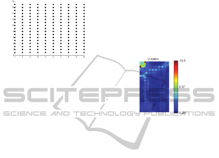
structure as the topology of the map as we can see in
the figure 2. A prototype vector is associated with
IJCCI2012-InternationalJointConferenceonComputationalIntelligence
608
each neuron.
Figure 2: Training map.
For training and visualization purposes, the
sample vectors are assigned to the most similar
prototype vector, or best-matching unit (BMU),
which means that input vectors which are relatively
close in the input space should be mapped to units
that are relatively close on the lattice. Once the map
has been trained, it is ready for post-processing and
evaluation.
In this study we have calculated the values of
annealing temperatures and speeds of the coil points
located every 10 meters and the average of these
values for each coil.
The input vector has the main variables that take
part in that annealing process. They are: annealing
calculated with Rec 1 equation, annealing calculated
with Rec2 equation, heating, top and bottom
temperatures of six zones, steel band speed, length,
wide and thickness. In that way, the vector is such as
[Stainless_steel_type Rec1Sup Rec1Inf Rec2Sup
Rec2Inf CalorSup CalorInf Output_temperature
Speed thickness Wide Length Z1Sup Z1Inf Z2Sup
Z2Inf Z3Sup Z3Inf Z4Sup Z4Inf Z5Sup Z5Inf
Z6Sup Z6Inf]. Due to the number and variety of data
for each type of steel coils we have decided to use a
few of them for training and the others for
validation.
Scaling of variables is of special importance in
the Toolbox. Typically, one would want the
variables to be equally important.
The number of units in each map is calculated
using a heuristic formula determined by the SOM
method. It is based on Map_units=5* dlen ^0.54321
* k where dlen represents the number of vectors
used in the training and k = 4 because a ‘big’ map
has been chosen. After the number of map units has
been determined, in this map 168, the map size is
fixed [17, 10]. Then the SOM is initialized by a
linear initialization along two greatest eigenvectors
tried. After initialization, the SOM is trained in two
phases: first rough training and then fine-tuning.
6 ANALYSIS OF RESULTS
We have built and trained a SOM neural network,
using real data coil measured in a production line in
the Acerinox factory in Algeciras.
The U-matrix displays distances between
neighboring map units, and shows the structure of a
cluster map: high values of the U-matrix indicate a
cluster border, uniform areas of low values indicate
clusters themselves. Each component plane shows
the values of one variable in each map unit.
Figure 3: U-matrix.
The result of training is shown in Figure 4. This
figure shows the matrix distances and projections of
each variables of the input space. This type of
network elements, called neurons, are arranged in a
two-dimensional network, each of these elements
will be calculated in the learning process of the
network. They are representatives of different states
of annealing, such as: excess, lack or correct
annealing. The objective of this type of network is to
determine relationships inherent in data according to
their relationships. So, our objective is to visually
determine relationships between the different
variables of interest in our study.
In figure 4, we can see the homogeneity of the
variables representing the temperature of the
annealing furnace. The left top colour blue
represents highest temperatures and corresponds to
highest values of annealing and the thickness of the
steel band. On the other hand, we also note that the
width and length have no real connection to the
others variables. Finally, the velocity tends to be
higher in cases of lower annealing and lower in
cases of higher annealing.
Two of the properties most of the measures of
SOM Quality try to evaluate are vector projection,
which is sometimes referred to as “topology
preservation”, and vector quantization. Technically,
there is a trade off between these two, increasing
projection quality usually decreases the projection
properties. The Quantization Error (QE) is computed
ANon-linealMathematicalModelforAnnealingStainlessSteelCoils
609

by determining the average distance of the sample
vectors to the cluster prototype vectors by which
they are represented. We have obtained a
quantization error of 0,985 and a topographic error
of 0,026. All entries area presented to SOM network
are assigned to a cluster. The Clustering process
groups those areas or clusters where the Euclidean
distance between adjacent vectors is lesser
(Kohonen, 1997). To measure how an entry point
belongs to the cluster it has been assigned to, the
quantization error can be used. This error is
calculated as the Euclidean distance between the
inlets to the vector of the neuron is activated.
Figure 4: Projections of each variable of the input space.
Figure 5: Clusters.
Finally, the structure is chosen optimal using the
Davies-Bouldin index considering both the distance
between clusters as internal distance of each cluster.
The red zone represents the coils that have less
heating than required, the yellow zone the well
annealing coils and the blue zone represents the coils
with excess of heating ant the dark blue the rest.
7 CONCLUSIONS
An alternative and successful approach has been
introduced based on neural networks for
classification of data series and it has been applied to
the classification of annealing data acquired in a
stainless steel production line. The main results
obtained in this investigation are: An improved
clustering algorithm that generates clusters including
all the annealing neurons. The creation of SOM has
been improved by means of a better quality of the
training data and so a successful classification of
annealing stainless steel has been got.
At the moment we have centred on the global
classification of coils but we can’t characterize what
kind of abnormality it is affected for. Additional
work is necessary to do in this field and a supervised
neural network is proposed to use it in future
investigations. This study will be continued in a
thesis with a more detailed analysis and we will
contrasted SOM method with other techniques that
could also be employed in this scenario.
REFERENCES
Chapple Mike, “Data Mining: An Introduction”, 2002.
http://databases.about.com/library/weekly/aa100700a.
htm
J. Kangas, T. Kohonen, (1997). Developments and
applications of the self organizing map (SOM) and
related algorithms. Mathematics and Computers in
simulation, 41 (1-2); 3-12.
Khan S. H., Ali F., Nusair Khan A., Iqbal M. A., (2008).
Eddy current detection of changes in stainless steel
after cold reduction. Computational Materials Science,
vol.43, no.4, 2008, pp. 623-8.
T. Kohonen (1997) The Self Organizinf Map. Springer. 2ª
Ed.
T. Kohonen, J. Hunniyen, J. Kangas, J. Laaksonen, (1992-
1997). The Self Organizing Map program package”.
Helsinki University of Technology, Finland.
Reed, R. J., (2003). North American Combustion
Handbook. North American Manufacturing Company.
Cleveland.
C. Spinola, J. Bonelo, J. Vizoso et al., (2008). Supervision
model for the annealing process in a stainless steel
production line. IEEE International Conference on
Industrial Technology. Pages 1-4.
C. Spinola, J. Bonelo, J. Vizoso et al., (2004). An
approach to the analysis of thickness deviations in
stainless steel coils based on self-organising map
neural networks. Springer London. Pages 309-315.
DOI: 10.1007/s00521-004-0426-z.
Ben Young, (2008). Experimental and numerical
investigation of high strength stainless steel structures.
Journal of Constructional Steel Research, vol.64,
no.11, 2008, pp. 1225-30.
IJCCI2012-InternationalJointConferenceonComputationalIntelligence
610
