
Cost Functions for Scheduling Tasks in Cyber-physical Systems
Abhinna Jain, C. M. Krishna, Israel Koren and Zahava Koren
Electrical and Computer Engineering, University of Massachusetts, Amherst, MA 01003, U.S.A.
Keywords:
Cyber-physical Systems, Task Scheduling, Cost Functions, Controlled Plant Dynamics.
Abstract:
In Cyber Physical Systems (CPS), computational delays can cause the controlled plant to exhibit degraded
control. The traditional approach to scheduling in such systems has been to define controller task deadlines,
based on the dynamics of the controlled plant. Controller tasks are then scheduled to meet these deadlines;
meeting the deadline is considered the sole criterion for scheduling success.
This traditional approach has the advantage of simplicity, but overlooks the fact that the quality of control
depends on the actual task response times. Two different schedules, each satisfying the task deadlines, can
provide very different levels of control quality, if their task response times are different.
In this paper, we consider using cost functions of task response time to capture the impact of computational
delay on the quality of control. Since the controller workload typically consists of multiple tasks, these cost
functions are multivariate in nature. Furthermore, since these tasks are generally coupled, the response time
of one control task can affect the sensitivity of the controlled plant to the response times of other tasks.
In this paper, we first demonstrate how a multivariate cost function can be formulated to quantify the effect of
computational delays in vehicles. We then develop cost-sensitive real-time control task scheduling algorithms.
We use as an application example an automobile: the controller workload consists of steering and torque
control. Our results indicate that cost-function-based scheduling provides superior control to the traditional
deadline-only-based approach.
1 INTRODUCTION
Modern control systems such as automobiles, aircraft,
missiles and robots rely more than ever on computers
for their control. In such applications, the computer
is in the feedback loop of the controlled plant. It gen-
erates appropriate actuator outputs in response to sen-
sor and user inputs. The aim is generally to optimize
some specified performance functional (e.g., time, en-
ergy, or distance from intended target or trajectory)
over the course of a given mission.
Both fixed and adaptive approaches have been
used for launching tasks in the control computer.
In the fixed case, tasks run periodically. Typically
zero-order hold is used, holding the actuator output
fixed between successive updates. In the adaptive ap-
proach, control tasks are generated either by event
triggering or self-triggering. In event-triggering, the
state of the controlled plant is monitored, and given
computational tasks are launched if the plant en-
ters some pre-determined subset of its state-space
(Tabuada, 2007; Vasyutynskyy and Kabitzh, 2010).
In self-triggering, it is the job of a task iteration
to specify when the next iteration is to be issued
(S. Samii and Cervin, 2010; Wang and Lemmon,
2009).
Clearly, these approaches can be combined. For
example, one may have regular tasks running pe-
riodically to control a chemical reactor, and at the
same time, appropriate corrective tasks (like opening
a safety valve or turning down the temperature) may
be triggered if the pressure in the reactor vessel ex-
ceeds a given value.
The typical approach to scheduling such tasks is
deadline-centric. Each control task has a deadline as-
sociated with it; scheduling algorithms such as Rate
Monotonic (RM) or Earliest Deadline First (EDF) can
be used to ensure that deadlines are met. If deadlines
are associated with task graphs rather than individual
tasks, virtual deadlines are usually associated with the
individual tasks in order to allow traditional deadline-
based scheduling protocols to be used.
Task deadlines are obtained by considering the dy-
namics of the controlled plant. One considers the time
available before the controlled plant state enters some
dangerous state.
The implicit assumption in deadline-centric
scheduling is that as long as the deadlines are met,
the quality of control provided is adequate; sometimes
when the jitter caused by an abnormally early execu-
412
Jain A., M. Krishna C., Koren I. and Koren Z..
Cost Functions for Scheduling Tasks in Cyber-physical Systems.
DOI: 10.5220/0004046704120421
In Proceedings of the 9th International Conference on Informatics in Control, Automation and Robotics (ICINCO-2012), pages 412-421
ISBN: 978-989-8565-21-1
Copyright
c
2012 SCITEPRESS (Science and Technology Publications, Lda.)

tion is unacceptable, the system can artificially delay
the output by buffering. This is a pass/fail approach; a
task passes if it meets its deadline and fails otherwise.
The (considerable) advantage of such an approach is
its relative simplicity. The disadvantage is that it fails
to take into account the finer-grained dependence of
the quality of control on the actual controller delays.
To deal with this issue, a basic cost-function
approach to real-time workloads was introduced in
(Krishna and Shin, 1983; Krishna and Shin, 1987;
K.G. Shin and Lee, 1985). That work introduced
the notion of a cost function to capture the impact of
feedback delay in a single, isolated, control task, on
the performance of a controlled plant; one case study
used was that of elevator control during the land-
ing flare of an aircraft. In follow-on work, a simple
heuristic was introduced to schedule with such cost
functions (Hegde and Krishna, 1994). This work fo-
cused on univariate cost functions. That is, the cost
associated with a certain controller delay with respect
to an individual task was independent of the delays
suffered by other tasks.
In the present work, we extend this approach to
consider multivariate cost functions. We first intro-
duce these cost functions, using as a case study the
steering and torque control tasks of a car, for which
we illustrate some issues related to multivariate cost
functions. A key issue is the fact that control tasks
are coupled; the delay suffered by one task affects the
sensitivity of another task to controller delay. Fur-
thermore, cost functions depend on the control proto-
cols followed (e.g., what algorithms are used to com-
pute the actuator input and whether zero-order or first-
order hold is used), so that a library of control sit-
uations needs to be constructed. The actual control
”trajectory” of a plant can be created by a piecewise
composition of these elements. For example, one
can break down a car’s trajectory approximately into
straight lines and arcs; in each, certain cost functions
apply to the steering and torque tasks.
In the second part of the paper we introduce
uniprocessor scheduling heuristic algorithms to min-
imize a general multivariate cost function. Offline
scheduling algorithms are used to generate template
schedules based on the worst-case execution times
(WCETs) of the tasks. Lightweight online schedulers
update these templates when tasks complete ahead of
their WCETs.
2 MULTIVARIATE COST
FUNCTIONS
Several factors affect the performance of a controlled
plant. Some of these are:
• Quality of the control algorithm, e.g., the kind of
optimization used, whether model predictive con-
trol (Camacho and Bordons, 2003) is used, etc.
There can sometimes be a tradeoff between the
quality of the algorithm and the time overhead it
imposes.
• Sensor sampling rate and the associated frequency
of the various control tasks. The sensor rate is de-
termined by evaluating the dynamics of the sensed
variables; the control task frequency is determined
by studying the dynamics of the controlled plant.
• Control applied between updates of the control
output, e.g., zero-order hold (ZOH), first-order
hold (FOH), predictive first-order hold (PFOH)
(Astrom and Wittemark, 1997; Kuo, 1992).
• Feedback delay.
In this paper, we focus on the feedback delay: the
impact it has on the controlled plant performance,
and how to schedule activity on the control computer
while keeping this impact in mind. We will focus here
on a periodic control task workload. It is not difficult
to extend this work to event-triggered or self-triggered
tasks.
Feedback delay depends on the execution time of
the various control tasks. In order to evaluate the
schedule feasibility (i.e., does it meet deadlines) and
quality, we need estimates of the worst-case execution
time (WCET) and also its distribution function. There
is a large and growing literature on obtaining WCETs
in real-time systems.
2.1 Definition of Cost Function
It is well known that feedback delay pushes the poles
of a controlled plant towards the right half-plane,
reducing its stability. Beyond a certain point, the
poles can cross into the right half-plane, rendering the
plant unstable. More generally, we assume the exis-
tence of a performance functional which captures the
application-relevant aspects of the control plant per-
formance (F.L. Lewis and Syrmos, 2012; Sage and
III, 1977). We assume that this is expressed in units of
cost rather than reward, i.e., the lower the functional
value, the better. The approximate impact of the con-
troller delay on this functional is the focus of the cost-
function approach. In what follows, we will use the
terms delay and response time interchangeably.
More precisely, let the control tasks be T
1
, ··· , T
n
.
Denote by F(x,ξ
1
, ··· , ξ
n
) the cost functional value
associated with the plant starting in state x over a
given residual period of operation, T
op
, and the as-
sumption that each iteration of task T
i
has response
CostFunctionsforSchedulingTasksinCyber-physicalSystems
413

time ξ
i
, for i = 1, · · · , n. Then, the cost function asso-
ciated with these response times is given by
C(x, ξ
1
, ··· , ξ
n
) = F(x, ξ
1
, ··· , ξ
n
) − F(x, 0, ·· · , 0)
(1)
Note that F() may be any functional that captures the
aspects of performance relevant to the user; no restric-
tion is placed on its form. Note further that this is only
defined when task response times do not exceed their
respective deadlines.
Remark 1: Since the plant state-space may be very
large, it is not practical to try to evaluate this cost
function at each point. Instead, one breaks down the
state-space into subspaces and associates a cost func-
tion associated with each subspace. This may be ob-
tained, for example, by selecting a certain number
of random samples over that subspace and averaging
the cost function values for those samples. The finer
the granularity of the division into subspaces and the
greater the number of samples taken, the more accu-
rately the cost functions reflect the actual behavior of
the system; however, this is at the cost of an increased
number of cost functions overall and more (offline)
computational work.
Remark 2: In reality, the response times of different
iterations of an individual task are certain to vary. To
obtain an exact characterization of the impact of the
delay of any individual iteration, we would have to
calculate the impact on the performance functional of
each of the response times of the thousands to mil-
lions of iterations executed over any reasonable pe-
riod of operation T
op
. This is clearly impractical, and
so in our calculations of the cost function we use a
single reference value, ξ
i
, for the response time as-
sociated with all iterations of an individual task, T
i
,
i = 1, · · · ,n. This cost function is then used as an ap-
proximation of the impact on the control plant per-
formance of task T
i
. Note that because the cost func-
tion is also a function of the plant state, which encom-
passes the impact of all the control delays up to that
point, this is an acceptable approximation.
Remark 3: If we are evaluating the total cost over
some given trajectory starting from some given point,
then we can drop the dependence on x and define the
cost function just in terms of the response times over
the period of operation. This is what we do in the ex-
amples in this paper.
Remark 4: The cost function is a multivariate func-
tion. We will see later that in many cases, cost func-
tions have cross terms such as ξ
i
ξ
j
for i 6= j. This
reflects the fact that the response time of one task can
affect the sensitivity of the plant to the response time
of another.
Remark 5: If the controlled plant operation has well-
defined distinct phases, each with its own demands
and task loading (e.g., in an aircraft - takeoff, cruise,
landing flare, landing), one can define cost functions
over these individual phases rather than over the entire
period of operation. If the plant operates essentially
forever, we can set any practical horizon (e.g., a day)
over which the performance functional is evaluated.
If a shorter time horizon is desired (e.g., just a few
seconds), that can be implemented as well. The point
is that our assessment of the impact of a nonzero con-
troller delay is entirely within the control of the user
and can respond fully to the particular needs of the
application.
Remark 6: We are assuming a traditional real-time
task model. In certain circumstances, one can have a
choice of which tasks to pick. Multiple tasks could be
available for the same control function, each with its
own characteristic computational resource (e.g., CPU
cycles, memory) requirements and a certain level of
output quality (e.g., how close to optimal it is, how
susceptible it is to failure caused by numerical insta-
bility). It is not difficult to extend our cost function
model to account for this.
2.2 Case Study: Car Control on a Curve
To understand some of the issues related to multi-
variate cost functions, we consider a case study in-
volving the control of a car. In particular, steering
and torque/braking inputs are provided to each of the
wheels of the car. The model we use is the four-
wheeled steering and four-wheeled drive (4WS4WD)
system modeled in (Peng, 2007).
In (Peng, 2007), the kinematics (study of the ve-
hicle body and wheel dynamics, taking into account
the tire friction) of a 4WS4WD car are modeled in
some detail. A bounded controller with integral com-
pensation is introduced. Our objective is to develop
cost functions associated with having the car track a
curved reference path. We use the same vehicle char-
acteristics as in (Peng, 2007): see Table 1 for the key
parameters (a full description can be found in (Peng,
2007)). The cost functional we chose as best con-
Table 1: Key Car Parameters (from (Peng, 2007)).
Mass 1480 kg
Inertial moment about vertical 1950 kg · m
2
Distance from CG to front 1.421 m
Distance from CG to rear 1.029 m
Effective width 1.502 m
Height of CG 0.42 m
veying the effect of computational delays (response
times) is the area between the reference car trajectory
and the actual trajectory followed by the car. Our aim
ICINCO2012-9thInternationalConferenceonInformaticsinControl,AutomationandRobotics
414

is to express this quantity as a multivariate analytic
function of the delays, and consequently, schedule the
car control tasks such that this cost is minimized.
Unless stated otherwise, our numerical results as-
sume a zero-order hold over the task period. Figure
1 shows the actual car trajectory for a holding period
of 200 ms and a variety of controller delays, ranging
from 0 to 170 ms. In order to limit the number of
curves in the figure, we set the delay of each of the
control tasks equal to this amount. Figure 2 shows
(as one would expect) that for the same controller de-
lay, operating the car at a higher velocity results in
a greater deviation from the desired trajectory, i.e., a
higher cost.
Figure 1: Car Trajectory for Various Controller Delays.
Figure 2: Car Trajectory for Different Velocities.
Let us consider, for simplicity of presentation, the
case where the four steering tasks (one to each wheel)
all have the same response time ξ
1
and the four torque
tasks have the same response time ξ
2
. We assumed a
15 m curve, and calculated the cost (i.e., the actual
area between trajectories) for different values of the
delays ξ
1
and ξ
2
. The results are shown in Figure 3.
Using curve-fitting software, we found the following
polynomial expression for the cost function for the
range of response times studied:
f (ξ
1
, ξ
2
) = 48.3 − 52.4ξ
1
− 141.1ξ
2
+ 1436.5ξ
2
1
+
1806.4ξ
2
2
− 2423.4ξ
1
ξ
2
(2)
Figure 3: Bivariate Cost Function.
Similarly, we used curve fitting to calculate analytical
cost functions for other reference trajectories and for
other velocities, and some of them are shown in Ta-
ble 2. We can now make the following observations:
• Both the reference (i.e., desired) trajectory and the
car speed play a large role in determining the cost
function; the cost functions are quite different for
different trajectories and speeds.
• Whether ZOH or FOH is used also has a substan-
tial impact on the cost of the task delays.
• In several instances, we have cross-terms, i.e.,
terms involving a product of x
1
and x
2
terms. This
indicates that the marginal performance of one
task is affected by the response time of the other.
• The actual trajectory of the car cannot obviously
be determined a priori. However, we can reason-
ably assume that it is composed of multiple seg-
ments, stitched together, and obtain various pos-
sibilities for each segment. At a minimum, two
types of segments: straight lines and arcs (of vary-
ing radii) are sufficient. Cost functions associ-
ated with each of these can be derived offline.
Scheduling can be done over each such segment:
since a car is a mechanical object, the duration of
each segment is obviously large with respect to
the control task periods. Each segment can there-
fore be treated as an individual phase in the op-
eration of the car. Offline task schedules for such
segments can be generated for standard segment
types; the one closest to the actual track selected
by the driver is used. A handful of such segments
is all that is required. For example, the cost func-
tion for a straight-line segment of length 40 m is
not very different from that of length 100 m. In
much the same way, for other controlled plants,
the period of operation can be divided into seg-
ments or phases.
We should emphasize that we assumed only two re-
sponse times, x
1
and x
2
, for ease of exposition. In the
general case, each of the four torque tasks and each of
CostFunctionsforSchedulingTasksinCyber-physicalSystems
415

Table 2: Cost Functions Comparison.
Radius of
ref. curve
(in m)
Period = 100 ms Period = 300 ms
ZOH FOH ZOH FOH
10 0.14x
0.13
1
x
0.74
2
3.59x
0.37
1
x
−0.31
2
58.8x
−0.34
1
x
0.14
2
3.9x
0.17
1
x
0.036
2
35 6.4x
0.12
1
x
0.15
2
5.6E − 07x
4.9
1
+
16.7x
0.25
2
0.92e
0.017x
1
+0.86E−04x
2
2
+
0.088x
1
11.74x
0.12
1
x
0.80
2
−
0.2E + 03
the four steering tasks can have a different execution
time; the cost function will then have eight response-
time arguments.
We next present a general model of our system
and the optimization problem we encounter. We later
suggest heuristic algorithms for solving the problem
and numerical results to evaluate the usefulness of our
algorithms.
3 SYSTEM MODEL
The notations are defined in Table 3.
Table 3: Notations.
p
i
Period of task i
d
i
Deadline of task i
w
i
Worst case execution time of task i
r
i
Remaining execution time of task i
U ≤ 1 - Utilization of uniprocessor
a
i,m
Arrival time of m
th
iteration of task i
f in
i,m
Completion time of m
th
iteration of
task i
ξ
i,m
Response time of m
th
iteration of
task i
H
Major period : LCM of all tasks’ pe-
riods
S
t
Task scheduled at time t
Z
j
Decision point : Arrival or comple-
tion time of a task
MC
i
Marginal cost for task i
A typical approach in scheduling involves assign-
ing tasks to processors and then scheduling the tasks
assigned to each processor. Following this approach,
we discuss in this paper a workload consisting of n
periodic tasks T
1
, T
2
, ... , T
n
executing on a uniproces-
sor system. Task T
i
has a deadline d
i
, a period p
i
, and
a worst case execution time w
i
(i = 1,..., n). The ac-
tual running time of the task follows some statistical
distribution in the interval (0, w
i
].
A task set is assigned to a processor such that its uti-
lization (U =
∑
n
i=1
w
i
p
i
) is less than or equal to 1 and
the task set is schedulable; Each schedule is gener-
ated over the major period (H) which is the LCM of
all task periods and is repeated every H time units.
We denote the task scheduled at time t by S
t
. A deci-
sion point at which the scheduler has to make a deci-
sion about which task to run next can be either a task
completion or a task arrival. This may involve pre-
emption of the task currently run. As is traditional in
real-time scheduling work, we assume that preemp-
tion costs are negligible. Denoting by L the number
of such decision points during the major period H, we
denote these points by Z
1
, ..., Z
L
.
Denoting by a
i,m
the arrival time and by f in
i,m
the
finishing time of the m
th
iteration of T
i
, then its re-
sponse time is ξ
i,m
= f in
i,m
− a
i,m
. The cost func-
tion associated with the tasks T
i
,..T
j
,..T
k
is represented
as f(ξ
i
, ..ξ
j
, ..ξ
k
) where tasks T
i
..T
j
..T
k
are dependent
and ξ
i
,..ξ
j
,..ξ
k
are their respective response times.
Our objective is to schedule the tasks such that the
total cost over H is minimized and all the tasks’ dead-
lines are met.
4 COST FUNCTION BASED
SCHEDULING ALGORITHMS
In this section we assume that the processor speed is
fixed, and describe a heuristic scheduling algorithm
consisting of two phases: offline and online. In the
offline phase, all the information about the tasks, in-
cluding their arrival times and their worst case exe-
cution times, is provided ahead of scheduling. In the
online phase, the algorithm uses the task order calcu-
lated by the offline phase and responds to the actual,
usually shorter, execution times of completed tasks by
assigning the reclaimed time to the task with the high-
est marginal cost at this point. An offline exhaustive
search for the optimal schedule is possible in theory,
but is prohibitively complex in practice. We there-
fore suggest first a fast greedy heuristic algorithm, and
then a slower Simulated Annealing based algorithm.
4.1 Offline Greedy Algorithm: GH
If tasks were independent, making scheduling deci-
ICINCO2012-9thInternationalConferenceonInformaticsinControl,AutomationandRobotics
416

sions would be fairly straightforward. Among all
available tasks, tasks would be scheduled in descend-
ing order of costs incurred. However, tasks are not in-
dependent, and the dependency of tasks through mul-
tivariate cost functions limits the total cost calculation
until the response times of all the correlated tasks are
known, which limits the scheduling decisions. For
example, if two correlated tasks, T
1
and T
2
, are in the
system at a time and no deadline constraints are vio-
lated, the scheduler has no basis of deciding whether
to schedule T
1
or T
2
first since it does not know their
response times and thus cannot compare costs. We
handle this problem by calculating, at every decision
point, the marginal cost of each of the tasks present at
this point - i.e., the partial derivative of the cost func-
tion w.r.t. the response time of each task. We then
select for execution the task with the highest deriva-
tive, since this will reduce our immediate cost by the
highest amount.
Our heuristic algorithm starts with a schedule gen-
erated by the Earliest Deadline First (EDF) schedul-
ing algorithm. While this is not cost-sensitive, it is
an optimal scheduling algorithm in terms of meeting
deadlines (Liu and Layland, 1973). The EDF sched-
ule provides an initial response time for all tasks,
which we then substitute in the partial derivatives of
the cost function to determine the task with the high-
est marginal cost. At every decision point, we swap
the currently scheduled task with the highest marginal
cost task based on current response times, as long as
deadlines are not missed. We then update the response
times of the tasks and move to the next decision point.
This is clearly a greedy approach, since it only con-
siders the local conditions at each scheduling point
rather than the whole period of operation.
Following is the pseudo-code for the greedy algo-
rithm, using as inputs a task set (TS) and a cost func-
tions set (CF):
Heuristic Offline Greedy(TS,CF)
// Latest response time of task i : ξ
i
// Vector ξ = (ξ
i
, ....., ξ
n
)
// L = Total no. of decision points
1. Run EDF to generate schedule S[]
2. // Cost optimization step
// Decision points Z
1
, ...., Z
L
, corresponding to arrival
and departure times, ordered temporally
ξ = (0,...,0)
for (j = 1; j ≤ L; j + +)
{
//(i)
Update ξ if departure happens at Z
j
Generate set of tasks available at Z
j
∀ i ∈ {1...n}
r
i
= remaining execution time o f task i at time Z
j
∀ i ∈ {1...n}, calculate
MC
i
=
∂C(x,t)
∂t
i
t = ξ
//(ii)
while (∃ MC
i
> 0)
{
k = arg max{
MC
i
MC
i
> 0}
S
current
[] = Tasks scheduled in the interval
[Z
j
, Z
j
+ r
k
]
// Swap T
k
and S
current
[]
S
0
[] = S[] after swap
if (Cost(S’[]) < Cost(S[])) && (no deadline
is missed)
{
S[] = S
0
[]
break
}
else MC
k
= 0
}
}
4.2 Online Time Reclamation
Since actual running times of tasks are generally
much smaller than their estimated worst case, there is
time to be reclaimed upon the completion of a task.
An online algorithm must be lightweight, so once
more we use the tasks’ marginal costs and select for
execution the task in the system with the highst partial
derivative of the cost function.
Following is the pseudo-code for our online time-
reclamation algorithm:
Given:
1. t
rec
is the time reclaimed upon completion of a task.
2. t is the current online time.
Heuristic Online(t
rec
,t)
if t
rec
== 0 , return
else
{
while t
rec
!= 0
{
Generate set of tasks available at time t.
Calculate marginal costs based on response
times from online if available (or) from offline
response times and pick T
k
with the highest
marginal cost
if A is not empty
{
CostFunctionsforSchedulingTasksinCyber-physicalSystems
417

count = min (time duration after t for which T
k
is alive , t
rec
)
t
rec
= t
rec
− count
}
else
return
} // while-end
}
4.3 Offline - Simulated Annealing - SA
The greedy algorithm GH described in Subsection 4.1
is geared towards minimizing the cost for the WCETs
of the tasks, while the actual running times (AET s)
are almost always much shorter. The lightweight on-
line algorithm has only limited time and ability to
adapt the schedule accordingly. We therefore gen-
eralize the online algorithm to target, rather than the
WCET s, a fixed percentage of the WCET s which can
be a user specified parameter, and can depend on the
statistical distribution of the AET s. To this end, we
take the following approach. We consider a priority
scheme which assigns priorities to each task in each
iteration. π
i,m
is the priority of task i in iteration m.
We then generate a schedule based on these priorities.
Note that the priority of a task may change from one
iteration to the next, unlike in a static priority scheme
like RM. We still ensure that all deadlines will be met
even if all tasks run to their WCET s.
We can now formulate the following optimization
problem: Assign priorities π
i,m
to each task iteration
over the major period H such that the expected cost
is minimized subject to the need to keep the dead-
lines satisfied even if every task runs to its WCET .
To solve this optimization problem, we use the well-
known Simulated Annealing algorithm. Following is
the pseudo-code explaining the algorithm in more de-
tail.
Heuristic Offline target perc WCET(TS,CF)
1. Assign static priorities in inverse order of finishing
times of the tasks from the EDF schedule
(SA takes these priorities as the starting point)
2. Generate schedules for the priority assignment:
(i) Generate S
W
assuming that it runs to its WCET
(ii) if no deadline miss occurs
Generate S
E
assuming that each task iteration
runs to its targeted execution times.
Calculate cost for S
E
3. Change priorities:
In the each step of SA, change the priority as-
signment by randomly swapping two priorities where
each iteration of each task has equal probability of be-
ing swapped.
4. if search is successful, SA will provide a better
solution, i.e., a feasible solution where cost of S
E
is
smaller and no deadline miss in S
W
.
else call the GH and use its solution
5 NUMERICAL RESULTS
Numerical results for the algorithms in Section 4 are
presented here. We have developed simulators in the
C programming language for the following purposes
:
1. Solving delayed differential equations to obtain
cost functions.
Inputs to the simulator are the initial value of the
vehicle system state variables, delay value for tasks,
holding period and time of travel. For a given time of
travel, the simulator calculates the cost corresponding
to the given delay values. The cost is calculated for
different combinations of delay values.
2. For implementing scheduling heuristics.
For implementing the scheduling heuristics, we
take a task set and cost functions as inputs and gen-
erate a schedule and cost value corresponding to that
schedule. A task set is generated for a specific utiliza-
tion/work load. It is generated by first randomly se-
lecting worst case execution times and periods from
a set and then normalizing them to achieve a specific
utilization value. The arrival time of the first iteration
of all the tasks (a
i,0
) is assumed to be at time zero,
the start of the schedule. For simplicity, we determine
the relative deadline of a task to be equal to its period,
so only one iteration of a task is alive at a time. We
assume that there is no scheduling and context switch-
ing overhead. AETs are generated based on a specific
statistical distribution. To calculate the total cost of
a schedule, we consider the latest response times of
tasks.
Extensive simulations were carried out to assess
the quality of our algorithms. We selected the number
of experiments such that the standard deviation of the
result was < 0.01, and the result is therefore stable
and reliable.
We tested our algorithms on two types of cost
functions; the car trajectory cost function, and an ar-
tificial cost function.
5.1 Cost Function for the Car
Trajectory
These numerical results were generated for 5 tasks in
ICINCO2012-9thInternationalConferenceonInformaticsinControl,AutomationandRobotics
418
the vehicle system considering individual steering on
all four wheels and a single torque task for the ve-
hicle. We derive a multivariate cost function as per
the discussion about cost functions in section 2.2, the
following cost function is obtained by curve-fitting:
e
ax
1
+bx
2
+cx
3
+dx
4
+ex
5
+ f
where x
1
is the
response time of the torque task, x
2
, x
3
, x
4
, x
5
are response times of steering task on the left front
wheel, right front wheel, left rear wheel, right rear
wheel, respectively, and a = 2.4, b = 1.2, c = 1.3, d =
1.26, e = 1.4, f = 2.3. We assumed a 10 m radius
of reference curve and holding periods of 150 ms
and 200 ms for torque and steering tasks, respec-
tively. For simulations, we randomly select WCETs
from set {5 − 60}ms and interleaved periods from set
{10, 20, 40, 80, 160}ms.
To check the quality of the resultant schedule (of-
fline followed by online), we obtain the vehicle trajec-
tory that would follow from this schedule. Therefore,
cost ratios shown in the results are ratios of the cost
obtained from the vehicle simulator. We call it final
cost/final cost ratio. This is needed to establish the
usefulness of the cost functions, to demonstrate that
they do indeed capture the control issues involved.
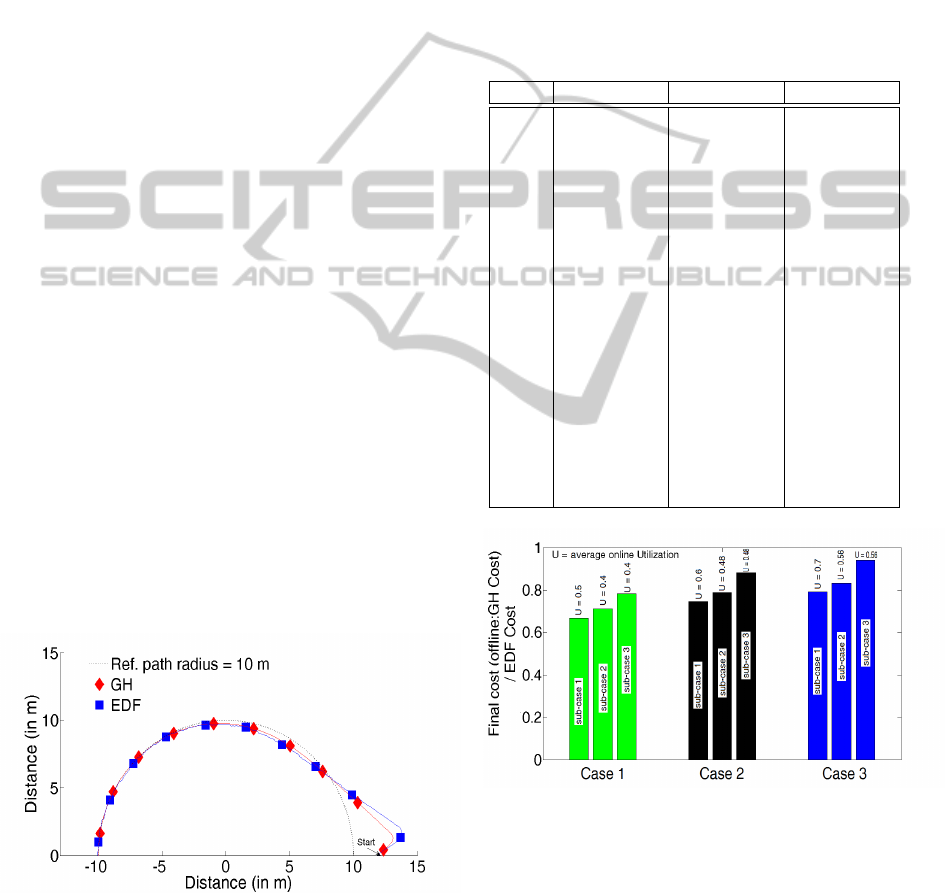
5.1.1 Example Trajectory
In Figure 4, we show an example of the comparison
between the result of EDF against the cost function
approach (GH) by showing the trajectory that results
in each case and calculating the total divergence
(between the reference and the actual tracks) for
each case. Task set has the online utilization of
0.52 and {WCET, period} of 5 tasks are as follows:
{20, 150},{40, 200},{40, 200},{40, 200},{40, 200}.
We can see that GH performs better than EDF by
about 25%.
Figure 4: Example - Trajectories for GH and EDF schedule.
5.1.2 EDF vs GH
Figure 5 compares the final costs of EDF and GH.
Each experiment consists of a different task set. AETs
are generated based on normal distribution with mean
= 80% of the WCET and standard deviation = (WCET
- mean)/2.
The plot shows variation of cost ratio with four
different cases. Each case shows three sub-cases. For
sub-case 1, average online utilizations for case 1,2,3
are 0.5,0.6,0.7, respectively. For sub-case 2 and sub-
case 3, average online utilizations in case 1,2,3 are
0.4,0.48,0.56, respectively. More details regarding
sub-cases are provided in Table 4:
Table 4: Section A - Greedy vs EDF cases description.
sub-case 1 sub-case 2 sub-case 3
case
1,2,3
Tasks run
to their
WCETs in
the online.
Online
heuristic
for GH is
nodvsONH
Tasks run to
their AETs
in the on-
line. Online
heuristic for
GH is nodv-
sONH
Tasks run to
their AETs
in the on-
line. Online
heuristic for
GH does
not sched-
ule tasks
with higher
marginal
cost during
reclaimed
time. It
simply run
next avail-
able task
or idle the
processor in
case no task
is available.
Figure 5: Vehicle cost function - Greedy vs EDF.
We observe that for sub-case 1, on the average
the GH final cost improves by about 27 % over the
EDF final cost, and for sub-case 2, this improvement
is about 22%. At higher utilizations, in the offline
phase, GH has less flexibility for making changes in
the schedule due to deadline constraints which results
in the poor offline result and thus higher final cost
compared to lower utilizations. Comparing sub-case
CostFunctionsforSchedulingTasksinCyber-physicalSystems
419

3 with sub-case 2 shows how the online algorithm per-
forms. As the utilization goes up, the offline GH is
poor, and the online has more room for online adjust-
ments. Our algorithms perform better than a simple
online heuristic which does not take advantage of the
reclaimed time. On the average, the online algorithm
improves the cost by around 10% .
5.1.3 GH vs SA
Obviously, the GH solution is not optimal. An opti-
mal algorithm would involve exhaustive search (mit-
igated by some pruning in a branch-and-bound ap-
proach), and is infeasible even for demonstration pur-
poses. Hence, to evaluate this algorithm, we use in-
stead an algorithm based on simulating annealing to
search for improvements over the output of our GH
algorithm. Our experiments shows 3 - 4% improve-
ment over the GH cost. A high temperature depreci-
ating factor for SA is chosen to allow it to cool down
slowly and search for a long duration. The fact that
SA only provides a small improvement despite a long
search attests to the quality of the GH approach.
5.1.4 Effect of Targeting Percentage of the
WCET
We observe an average improvement of about 10 -
15% in the online cost. Figures 6 and 7 describe the
effect of targeting some percentage of the WCET in
the offline over targeting WCET. The final cost ra-
tio is calculated for both cases for same AETs. We
use the following approach to generate synthetic task
workloads. AETs are generated based on a condi-
tioned normal distribution, whose mean lies halfway
between a specified percentage of WCET and WCET.
We select the standard deviation, σ, so that WCET
is 2σ away from the mean. Response times are gen-
erated using a normal random number generator; re-
sponse times that are either negative or outside the
range of 2σ from the mean are discarded.
In Figure 6, cost ratios are plotted for various of-
fline utilization values and for different values of the
mean and standard deviation. As σ decreases, the
quality of prior information we have about the AET
improves, and so our targeting heuristic performs bet-
ter. As the workload increases, less flexibility leads a
smaller improvement.
Figure 7 shows the impact of targeting a fixed per-
centage of the WCET at utilization of 0.6. We ob-
serve that if we target at values far from the average,
the improvement in the final cost is smaller than tar-
geting values closer to the average and for a normal
distribution of AETs, improvement in the final cost
Figure 6: Vehicle cost function - Final Cost Ratio:%WCET
vs WCET (Targeting values from a distribution).
Figure 7: Vehicle cost function - Final Cost Ratio:%WCET
vs WCET (Targeting fixed % of WCET).
is more when we target values obtained from a dis-
tribution compare to targeting fixed percentage of the
WCET.
5.2 Polynomial Cost Function
The heuristic algorithms presented above are general
and therefore applicable to a variety of cost func-
tions. We next demonstrate the use of our algorithms
for scheduling a system with 10 tasks and polyno-
mial cost functions. The WCET are selected from the
set {1 − 6} and the periods are selected from the set
{5, 10, 20, 40, 80}. The cost functions are as follows:
1st group cost function: f (x
1
, x
2
) = x
1
x
2
2
2nd group cost function: f (x
4
, x
5
) = x
3
4
x
5
3rd group cost function: f (x
6
, x
7
, x
8
) = x
6
x
2
7
x
8
4th group cost function: f (x
9
, x
10
) = x
2
9
x
10
Independent task cost function: f (x
3
) = x
2
3
where x
i
is the response time of T
i
.
In Figure 8 we observe a similar trend to that ob-
served for the vehicle cost function when comparing
GH and EDF.
ICINCO2012-9thInternationalConferenceonInformaticsinControl,AutomationandRobotics
420

Figure 8: Polynomial cost functions - Greedy vs EDF.
6 DISCUSSION
Cyber-physical systems have to work in two domains:
that of control and of computing. It is often quite
difficult to express the needs of the controlled plant
in terms meaningful to engineers on the computer
side. Traditionally, this has been done through defin-
ing deadlines and setting appropriate task invocation
periods by analyzing the dynamics of the controlled
plant. The job of the computer is then to manage its
resources in such a manner that all critical deadlines
are met. This is effectively a 0-1 criterion (meet/miss
deadlines) and can be well-handled by means of tra-
ditional real-time scheduling algorithms.
By contrast, in this paper, we have argued that
deadlines by themselves are only a first-order reflec-
tion of the needs of the controlled plant. A more de-
tailed consideration of the controlled plant dynamics
leads to cost functions, which quantify the degrada-
tion in control caused by computational latency. Since
we generally have multiple tasks, and these tasks are
effectively coupled in their effect on the controlled
plant, the cost function is usually multivariate with
cross terms. The cost function captures more detail
as to the needs of the controlled plant than does the
traditional set of hard deadlines.
We have presented simple algorithms for the
uniprocessor scheduling of tasks to improve the qual-
ity of control provided under a fixed-frequency ap-
proach. An obvious extension of this work is multi-
processor scheduling; this is the subject of our ongo-
ing research.
ACKNOWLEDGEMENTS
This work was partly supported by the National Sci-
ence Foundation under grant CNS - 0931035.
REFERENCES
Astrom, K. and Wittemark, B. (1997). Computer-
Controlled Systems. Prentice-Hall.
Camacho, E. and Bordons, C. (2003). Model Predictive
Control. Springer.
F.L. Lewis, D. V. and Syrmos, V. (2012). Optimal Control.
Wiley.
Hegde, U. and Krishna, C. (1994). Scheduling real-time
tasks with cost functions. In Journal of Information
Science and Technology, Vol. 4, No. 1, pp. 1–7.
K.G. Shin, C. K. and Lee, Y.-H. (1985). A unified method
for evaluating real-time computer controllers and its
application. In IEEE Transactions on Automatic Con-
trol, Vol. AC-30, No. 4, pp. 357–366.
Krishna, C. and Shin, K. (1983). Performance measures for
multiprocessor controllers. In Performance.
Krishna, C. and Shin, K. (1987). Performance measures
for control computers. In IEEE Transactions on Auto-
matic Control, Vol. AC-32, No. 6, pp. 467–473.
Kuo, B. (1992). Digital Control Systems. Oxford University
Press.
Liu, C. and Layland, J. (1973). Scheduling algorithms for
multiprogramming in a hard real-time environment. In
Journal of the ACM, Vol. 20, No. 1, pp. 4661.
Peng, S. (2007). On one approach to constraining the
combined wheel slip in the autonomous control of a
4ws4wd vehicle. In IEEE Transactions on Control
System Technology, Vol. 15, No. 1, pp. 168–175.
S. Samii, P. Eles, Z. P. P. T. and Cervin, A. (2010). Dy-
namic scheduling and control-quality optimization of
self-triggered control applications. In IEEE Real-Time
Systems Symposium, pp. 95–104.
Sage, A. and III, C. W. (1977). Optimum Systems Control.
Prentice Hall.
Tabuada, P. (2007). Event-triggered real-time scheduling
of stabilizing control tasks. In IEEE Transactions on
Automatic Control, Vol. 52, No. 9, pp. 1680–1685.
Vasyutynskyy, V. and Kabitzh, K. (2010). Event-based con-
trol: Overview and generic model. In IEEE Interna-
tional Workshop on Factory Communication Systems,
pp. 271–279.
Wang, X. and Lemmon, M. (2009). Self-triggered feedback
control systems with finite gain l2 stability. In IEEE
Transactions on Automatic Control, Vol. 54, No. 3, pp.
452–467.
CostFunctionsforSchedulingTasksinCyber-physicalSystems
421
