Two-view Epipole-based Guidance Control for Autonomous Unmanned

Aerial Vehicles

W. Achicanoy

, C. Sag¨u´es

, G. L´opez-Nicol´as

and C. Rodr´ıguez

Departamento de Ingenier´ıa Mec´anica, Universidad de los Andes, Bogot´a, Colombia

Departamento de Inform´atica e Ingenier´ıa de Sistemas, Instituto de Investigaci´on en Ingenier´ıa de Arag´on,

Universidad de Zaragoza, Maria de Luna 1, E-50018, Zaragoza, Spain

Keywords:

UAV Guidance, Epipolar Geometry, Nonlinear Engagement, Input-output Linearization, State Feedback.

Abstract:

A visual control based on epipolar geometry is proposed to guide an autonomous unmanned aerial vehicle

(UAV) to a target position. The interest of this contribution resides in a new controller that allows purely

vision-based guidance reducing the dependence on the accuracy of the system’s state estimation using sensors

as Inertial Measurement Units (IMU) and Global Positioning Systems (GPS). A current view and a target view

are deﬁned by a camera on-board the vehicle and a camera located at the target’s position, respectively. The

epipolar coordinates from these views are used todesign a nonlinear control based on input-output linearization

of the nonlinear engagement rule that relates the cameras’ positions in time. An integrator is included to force

the outputs (epipolar coordinates) to follow an equilibrium point and a state feedback control law is proposed

to stabilize the outcome of the linearized input-output mapping. Simulation experiments for guidance of an

small autonomous UAV with a classical three-loop autopilot are presented.

1 INTRODUCTION

UnmannedAerial vehicles (UAVs) are used in civilian

and military applications developing tasks of surveil-

lance and delivering cargo. Over the last decade,

UAVs have proved to be efﬁcient in several missions

around the world, motivating the aircraft industry in

improving their internal systems and their capabil-

ities. For example, a vision system could enable

UAVs tracking a large number of targets (Schneider-

man, 2012). The UAVs’ performance commonly de-

pends on aerial and ground operation centres and hu-

man assistance, but autonomous operation is neces-

sary for stand-alone missions, or when the commu-

nication links fail and the vehicle needs to switch

to a safe ﬂight mode. The accuracy of the UAVs’

ﬂight depends on the on-board sensors’ capabilities

and its control robustness; the navigation and guid-

ance systems usually use Inertial Measurement Units

(IMU) and Global Positioning Systems (GPS), to get

information of the self-position and self-attitude; on

the other hand, they use cameras, spectrometers, and

radars, to retrieve the target’s features, position and

attitude.

Cameras have been used in a wide range of appli-

cations for control of aerial, terrestrial, and aquatic

vehicles, and vision-based control has become a

special branch of research. Most of the research

on vision-based control for autonomous UAVs have

used cameras’ information, together with inertial and

global positioning sensors, as inputs for ﬁlters or esti-

mators. For example, a vision-based guidance based

on trajectory optimization is proposed in (Watanabe

et al., 2006) and the vision data is used for an EKF

to estimate the target’s position and velocity relative

to the vehicle. They include a cost function that min-

imizes the acceleration effort the vehicle demands to

accomplish with three independent missions: Target

interception, obstacle avoidance, and formation ﬂight.

In (Ma et al., 2007) a guidance law for a small UAV is

developed based on an adaptive ﬁlter that calculates

the target’s velocity over the image plane. The ﬁl-

ter only uses the tracking information of the moving

target and a control law regulates the vehicle’s yaw

rate at a constant altitude (no depth information is re-

quired).

From another point of view, visual-based con-

trol methods based on epipolar geometry and ho-

mography have been used for mobile robot naviga-

tion. (Mariottini et al., 2004) and (L´opez-Nicol´as

et al., 2008) have developed two-view visual-control

for nonholonomic robots by means of nonlinear con-

242

Achicanoy W., Sagüés C., López-Nicolás G. and Rodríguez C..

Two-view Epipole-based Guidance Control for Autonomous Unmanned Aerial Vehicles.

DOI: 10.5220/0004032402420248

In Proceedings of the 9th International Conference on Informatics in Control, Automation and Robotics (ICINCO-2012), pages 242-248

ISBN: 978-989-8565-22-8

 2012 SCITEPRESS (Science and Technology Publications, Lda.)

trol and tracking of epipoles signals. In (L´opez-

Nicol´as et al., 2010) both epipolar geometry and ho-

mography matrix are used to design separated con-

trols that are switched using information of the de-

generacy of the fundamental matrix. Epipole-based

control is used at the initial stage of the navigation,

whereas homography-based control is used at the end

(short baseline). Homography has been used for UAV

navigation in (Hu et al., 2007b), where a multi-view

visual-based control, that uses quaternions and ho-

mography between pre-recorded satellite images and

the vehicle’s actual images, is proposed to track a de-

sired trajectory over the earth. Given that the esti-

mated position is up to scale and the depth is un-

known, open problems in this approach are clariﬁed

in (Hu et al., 2007a). In (Kaiser et al., 2010) a multi-

view visual-based estimator based on homography

and GPS measurements is designed; using this infor-

mation an autopilot commands the vehicle’s control

surfaces. This estimator deals with two main chal-

lenges: The continuous tracking of features, entering

and leaving the vehicle’s camera Field of View (FoV),

and the GPS failures.

Given that the epipolar geometry has reported

successful outcomes in mobile robots, in this paper

we presented the development of a new controller

based on epipolar geometry for the guidance of an au-

tonomous UAVs with a single camera on-board is de-

veloped. The vehicle motion is assumed to be planar.

Two views, the current view (vehicle’s camera) and

the target view (static camera at the target’s position),

are used to compute the epipoles and to steer the vehi-

cle to a desired position. As in (Mariottini et al., 2004)

and (L´opez-Nicol´as et al., 2008), input-output lin-

earization (Khalil, 2002) is used, but on the cameras’

nonlinear engagement rule. The linearized output is

stabilized by an appropriated state feedback control

law and the outputs (epipolar coordinates) are forced

to follow an equilibrium point by means of an integra-

tor, that eliminates the steady state error and improves

the robustness of the closed-loop system. Both epipo-

lar coordinates in the current and target views are in-

dependently chosen as outputs. To deal with the com-

plexity of the aerial vehicle model, a classical three-

loop autopilot (Zarchan, 2007) is used to command

the vehicle. The controller reduces the complexity of

the on-board electronics, and the fact that only epipo-

lar estimation is required, makes it suitable for sim-

ple guidance applications. The paper is organized as

follows: in section 2 the planar epipolar geometry is

shown; in section 3 a state space representation of the

nonlinear planar engagement rule is presented; in sec-

tion 4 the control strategy is developed; and in section

5 results of the simulation experiments are analyzed.

Earth surface line

Inertial frame

Baseline

(Line of Sight LoS)

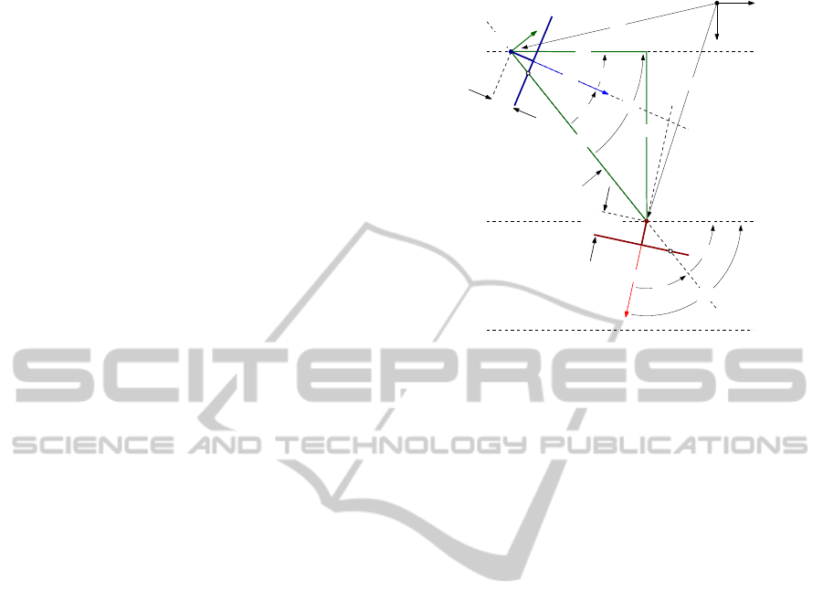
Figure 1: Planar two-view epipolar geometry (plane xz).

2 PLANAR EPIPOLAR

GEOMETRY

Figure 1 shows the planar two-view epipolar geom-

etry, relative to the inertial reference frame A, for

the autonomous UAV guidance problem. The ﬁrst

view is deﬁned by a current camera C

on-board the

vehicle, that is aligned with a current velocity vec-

tor v

= [u

]

and is located at a current posi-

tion p

= [x

]

, while the second view is an im-

age previously deﬁned by a target camera C

, that

is aligned with a target velocity v

= [u

]

at a

position p

= [x

]

. The epipoles e

∈ R

(cur-

rent) and e

∈R

(target) are subject to the constraints

= 0 and F

= 0, where F ∈ R

3×3

is the fun-

damental matrix. F is estimated from a set of fea-

tures correspondences using the RANSAC algorithm

(Hartley and Zisserman, 2004). These epipoles can

be written as e

= [e

c,w

c,h

]

and e

= [e

t,w

t,h

]

where (e

c,w

t,w

) and (e

c,h

t,h

) are the coordinates

(in pixels) along the image’s width and height, re-

spectively. For planar guidance design, only the co-

ordinates (e

c,h

t,h

) are useful, and it follows that

c,h

= f

tan(λ −γ

) (1a)

t,h

= −f

tan(γ

−λ) , (1b)

where f

and f

are the focal lengths for the current

camera and the target camera, respectively; λ is the

Line of Sight (LoS) angle, that is measured between

the LoS and the a

-axis; and γ

and γ

are the ﬂight

path angles for the current camera and the target cam-

era, respectively. These angles are measured between

the velocity vectors (v

and v

) and the a

-axis. By

deﬁnition the baseline is equal to the LoS.

Two-viewEpipole-basedGuidanceControlforAutonomousUnmannedAerialVehicles

243

3 PLANAR ENGAGEMENT RULE

The planar engagement rule is a description of the

evolution of the LoS angle λ and the LoS rate of

change

λ according to a lateral acceleration command

. If n

is proportional to

λ, then, the current cam-

era C

(vehicle) can be steered to the target camera

(target). This is the intuitive Proportional Nav-

igation (PN) (Yanushevsky, 2007). From Fig. 1,

λ = arctan(z/x), whit x = x

−x

and z = z

−z

and the LoS rate of change is

λ =

˙zx−z˙x

, (2)

where r =

√

+ z

is the magnitude of the instan-

taneous separation (range) between C

and C

. If

(2) is differentiated again, taking into account that

cosλ = x/r and sinλ = z/r, it follows that

λ =

¨zcosλ− ¨xsinλ

−

2˙r˙zcosλ + 2˙r˙xsinλ

. (3)

Given that C

is static, the C

’s acceleration com-

ponents, in terms of the lateral acceleration magnitude

, are ¨x = −n

sinλ and ¨z = n

cosλ, then, (3) can be

sympliﬁed as

λ = ωsin(λ −φ)+ n

/r , (4)

where ω = 2(v

/r)

and φ = arctan(˙z/˙x). v

= −

r is

commonly known as the closing velocity. Finally, the

planar engagement can be presented as the continuous

nonlinear system

η = f(η,u) =



ωsin(η

−φ)+ u/r



, (5)

where η = [η

,η

]

= [λ,

λ]

∈R

is the state vector,

u = n

∈ R is the input, and f(η,u) : R

×R → R

a vector ﬁeld.

4 EPIPOLE-BASED GUIDANCE

CONTROL

In this section, a guidance control based on input-

output linearization of the engagement system (5) is

presented. The output is based on the epipolar coordi-

nates’ measurements from the two images. The con-

trol law has the form of state feedback with integral

action. Both, the coordinate e

c,h

, deﬁned by the Eq.

(1a), and the coordinate e

t,h

, deﬁned by the Eq. (1b),

can be independently used as outputs, i.e., y = e

c,h

y = e

t,h

. If y is differentiated until the input u becomes

explicit it results that the relative degree of the system

(5) is 2, for all η ∈R

. We also obtain that either

u = −rωsin(η

−φ) −2r(η

−

)

tan(η

−γ

)

+ r

rcos(η

−γ

)

/ f

(6)

for y = e

c,h

, or

u = −rωsin(η

−φ) + 2rη

tan(γ

−η

)

rcos(γ

−η

)

/ f

v ,

(7)

for y = e

t,h

, lead the nonlinear output to the linearized

mapping

= ξ

= v

σ = e ,

(8)

where ξ

= y, ξ

= ˙y, v is the new control, and

e = ξ

−ξ

= y −y

is the output error. An integral

action was included in (8) forcing the output y to fol-

low a reference ξ

= y

. It is easily veriﬁed that the

augmented system (8) with realization





0 1 0

0 0 0

1 0 0















1 0 0



(9)

has a controllable pair (A

), and a state feedback

control

v = −K[ξ,σ]

, (10)

where K = [k

], can stabilize it. K is cho-

sen such that the matrix (A

−B

K) is Hurwitz (pole

placement) (Khalil, 2002) and local stability is guar-

anteed.

5 SIMULATION EXPERIMENTS

AND ANALYSIS

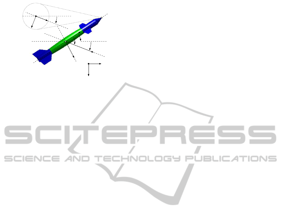
Figure 2 shows the model of an UAV, without propul-

sion and with a camera on-board, used to evaluate

the guidance control. For simplicity, a wing-body-tail

conﬁguration with a horizontal control surface (wing)

and a stabilizing ﬁxed surface (tail) was selected. Fast

control is guaranteed by means of the wing’s deﬂec-

tion angle δ, even though nonlinearities and rear sta-

bility interferences might appear (Chin, 1961). Given

that the downrange is limited, the earth is assumed to

be ﬂat. Three reference frames are deﬁned: (i) The

ICINCO2012-9thInternationalConferenceonInformaticsinControl,AutomationandRobotics

244

Vehicle

Camera

Figure 2: Autonomous UAV. The reference frames in the

vertical plane xz are: A (inertial), B (vehicle-ﬁxed), and C

(camera-ﬁxed).

inertial frame, named A, located at an initial altitude

; (ii) the vehicle-ﬁxed frame, named B, aligned with

the principal axes; and (iii) the camera-ﬁxed frame,

named C, aligned with the vehicle’s velocity vector

v or aero-stabilized. The camera’s principal axis is

parallel to the c

-axis and it is in the apex of the nose.

The rotation and translation equations can be found in

(Siouris, 2004). The estimation of the aerodynamic

coefﬁcients was computed using the Vortex Lattice

Method (VLM) (Melin, 2000). For simplicity, the

drag, lift and pitch coefﬁcients depend only on the

scheduling variables h (altitude) and M (Mach num-

ber) and are stored in look-up tables.

A classical three-loop autopilot (gyro and accel-

eration feedback), that translates acceleration com-

mands u to wing deﬂections δ is also used. A com-

plete description of the autopilot and the design equa-

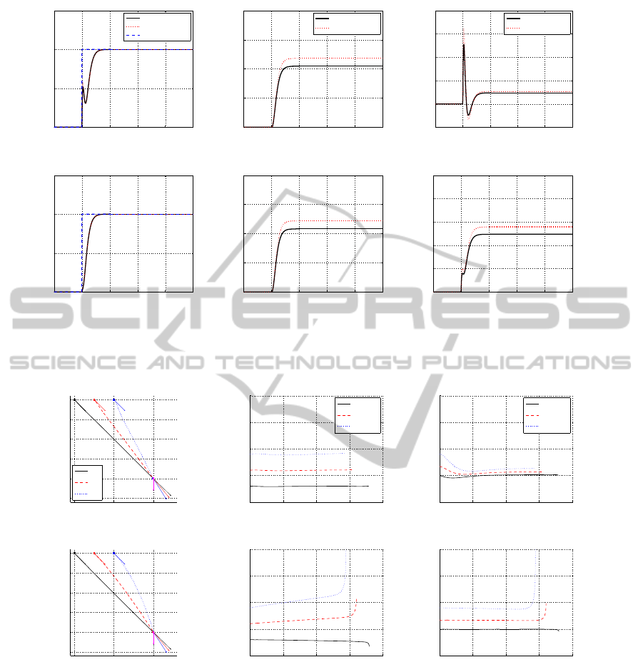
tions can be found in (Zarchan, 2007). Fig. 3 shows

the autopilot outputs for the step acceleration com-

mand u = u

(t −1) G (u

is the unitary step function),

for the ﬂight conditions h = 0 m (black continuous

lines), h = 1000 m (red dotted lines), M = 0.3, and

M = 0.9. The actuator’s dynamics are neglected and

ideal sensors are assumed. The design parameters are

= 50 rad/s (crossover frequency measured at the

gain margin), ζ = 0.7 (total acceleration damping),

and τ = 0.2 s (total acceleration time constant). Fig.

3(a) and Fig. 3(d) show the correspondence between

the desired acceleration n and the autopilot’s response

for these parameters. It is noted that the vehicle’s high

manoeuvrability is reached at low altitude h and high

Mach number M, and the angle of attack α and the

deﬂection angle δ stay at low values (Fig. 3(e) and

Fig. 3(f), respectively). For M ≤ 0.3 the autopilot

demands high values of α and δ (Fig. 3(b) and Fig.

3(c), respectively), and the vehicle’s aerodynamic ca-

pabilities are exceeded. This ﬂight condition can lead

the system to instability. In order to deal with the

change of the vehicle’s parameters, according to the

ﬂight conditions, a look-up table (with linear inter-

polation) is implemented to select the autopilot gains

according to the values of h and M.

On the other hand, it is assumed that the cameras

and C

are identical, ideal (skew is zero), and with

intrinsic parameters deﬁned as in (Hartley and Zis-

serman, 2004). The image resolution is 480 ×640

pixels, the focal length is f = f

= f

= 240 pixel,

and the epipoles’ measurements are assumed to be

known only from geometric relationships. For the

simulations, the frame A is ﬁxed at the initial alti-

tude h

= 2500 m, the vehicle’s initial velocity is

= 200b

m/s, and the initial attitude angle θ is

equal to the current cameraC

’s attitude angle γ

, i.e.,

the initial angle of attack α

= 0 deg. The state feed-

back control gain K is calculated with the Acker’s for-

mula.

Initially, it is shown that the control with unforced

output y, for both control laws (6) and (7) can be con-

sidered as PN-based control. This is explained by

means of the differentiation of the Eq. (1b), that re-

sults in a directly proportional relationship between

the rate of change of the target epipolar coordinate

˙e

t,h

and the LoS rate of change

λ. As in PN, the feed-

back of ˙e

t,h

multiplied by an appropriate constant can

stabilize the linearized output (8), which means that

the LoS angle λ is constant and the control based on

y = e

t,h

can drive the vehicle to the target position

(parallel navigation). An exact estimation of v

not necessary. Furthermore, if the vehicle’s path an-

gle γ

is replaced by a constant value, then, the differ-

entiation of the Eq. (1a) results in a directly propor-

tional relationship between ˙e

c,h

and

λ, and the control

based on y = e

c,h

is able to drive the vehicle to the

target position too. Fig. 4 shows the outputs of both

control laws for three different initial current cameras

c,1

at p

c,1

= [0, 0]

m, C

c,2

at p

c,2

= [500,0]

m, and

c,3

at p

c,3

= [1000, 0]

m. The initial attitude an-

gle is θ

= 45 deg for all the cameras. Fig. 4(a) and

Fig. 4(d) show that all cameras converge to the target

camera C

at p

= [2000,2000]

m (γ

= 90 deg) for

y = e

t,h

and y = e

c,h

, respectively. The gain K is the

same for both control laws and differences between

them are mainly noted in the shape of the trajecto-

ries. Fig. 4(b) and Fig. 4(f) show that the epipolar

coordinates e

t,h

and e

c,h

reach equilibrium points for

both control laws. Fig. 4(c) and Fig. 4(e) show the

free evolution of e

c,h

and e

t,h

for both control laws.

The shape of the vehicle’s trajectory is deﬁned by the

shape of the output epipolar coordinates. Fig. 5(a)

and Fig. 5(d) show the control action u (command

acceleration required for the three cameras C

c,1

, C

c,2

and C

c,3

) for both control laws. At the initial stage

of the guidance, a maximum acceleration effort is re-

quired for both control laws. However, the control

Two-viewEpipole-basedGuidanceControlforAutonomousUnmannedAerialVehicles

245

0 1 2 3 4 5

0.5

1.5

Time: t s

Lateral acceleration: n G

n (h = 0 m)

n (h = 1000 m)

(a) n (M = 0.3)

0 1 2 3 4 5

Time: t s

Angle of attack: α deg

α (h = 0 m)

α (h = 1000 m)

(b) α (M = 0.3)

0 1 2 3 4 5

−20

Time: t s

Deflection angle: δ deg

δ (h = 0 m)

δ (h = 1000 m)

0 1 2 3 4 5

0.5

1.5

Time: t s

Lateral acceleration: n G

(d) n (M = 0.9)

0 1 2 3 4 5

0.5

1.5

Time: t s

Angle of attack: α deg

(e) α (M = 0.9)

0 1 2 3 4 5

0.2

0.4

0.6

0.8

Time: t s

Deflection angle: δ deg

(f) δ (M = 0.9)

Figure 3: Autopilot response to step acceleration u = u

(t −1) G (blue dashed lines) at altitudes h = 0 m (black continuous

lines) and h = 1000 m (red dotted lines). The ﬁrst and second rows show the outputs for the Mach numbers M = 0.3 and

M = 0.9, respectively.

0 1000 2000

500

1000

1500

2000

2500

Downrange: x m

Crossrange: z m

c,1

c,2

c,3

(a) Trajectories (y = e

t,h

)

0 5 10 15 20

−300

−200

−100

100

Time: t s

Target coordinate: e

t,h

pixel

t,h

c,1

)

t,h

c,2

)

t,h

c,3

)

(b) e

t,h

(y = e

t,h

)

0 5 10 15 20

−100

100

200

300

Time: t s

Current coordinate: e

c,h

pixel

c,h

c,1

)

c,h

c,2

)

c,h

c,3

)

c,h

(y = e

t,h

)

0 1000 2000

500

1000

1500

2000

2500

Downrange: x m

Crossrange: z m

(d) Trajectories (y = e

c,h

)

0 5 10 15 20

−300

−200

−100

100

Time: t s

Target coordinate: e

t,h

pixel

(e) e

t,h

(y = e

c,h

)

0 5 10 15 20

−100

100

200

300

Time: t s

Current coordinate: e

c,h

pixel

(f) e

c,h

(y = e

c,h

)

Figure 4: Outputs of the guidance based on both output y = e

t,h

and output y = e

c,h

, for the three current cameras C

c,1

, C

c,2

and C

c,3

, positioned at different space locations but with the same initial attitude angle θ

= 45 deg. The ﬁrst and second rows

show the outputs for y = e

t,h

and y = e

c,h

, respectively.

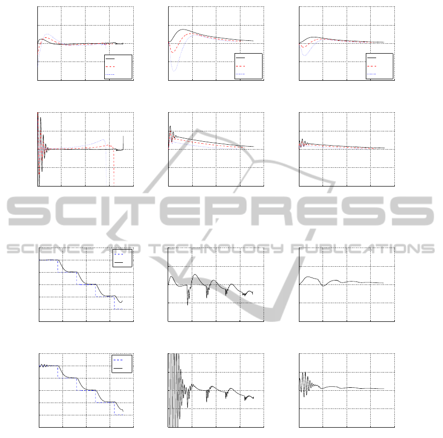
law based on the coordinate e

c,h

requires more accel-

eration than the control law based on the coordinate

t,h

. Control based on e

t,h

does not develop high am-

plitude oscillations at the initial stage of the guidance,

but it needs high values of α and δ. Fig. 5(b) and Fig.

5(e) show the angle of attack α, and Fig. 5(c) and

Fig. 5(f) show the deﬂection angle δ, for both control

laws. After the initial stage of the guidance, the val-

ues of the angles α and δ required for the control law

based on y = e

c,h

are smaller than the values required

for the control law based on y = e

t,h

. The camera C

c,3

requires the highest values of u, α and δ, due to its

initial condition; it is ahead of the other cameras and

needs more turning effort.

Next, the outputs y = e

t,h

and y = e

c,h

, are forced

to follow an equilibrium reference. Fig. 6(a) and

ICINCO2012-9thInternationalConferenceonInformaticsinControl,AutomationandRobotics

246

0 5 10 15 20

−10

−5

Time: t s

Lateral acceleration: u G

u (C

c,1

)

u (C

c,2

)

u (C

c,3

)

(a) u (y = e

t,h

)

0 5 10 15 20

−10

−5

Time: t s

Angle of attack: α deg

α (C

c,1

)

α (C

c,2

)

α (C

c,3

)

(b) α (y = e

t,h

)

0 5 10 15 20

−10

−5

Time: t s

Deflection angle: δ deg

δ (C

c,1

)

δ (C

c,2

)

δ (C

c,3

)

t,h

)

0 5 10 15 20

−10

−5

Time: t s

Lateral acceleration: u G

(d) u (y = e

c,h

)

0 5 10 15 20

−10

−5

Time: t s

Angle of attack: α deg

(e) α (y = e

c,h

)

0 5 10 15 20

−10

−5

Time: t s

Deflection angle: δ deg

(f) δ (y = e

c,h

)

Figure 5: Acceleration u, angle of attack α, and deﬂection angle δ for the set of current cameras C

c,1

, C

c,2

, and C

c,3

. The ﬁrst

and the second rows correspond to the controls based on y = e

t,h

and y = e

c,h

, respectively.

0 5 10 15 20

−50

−40

−30

−20

−10

Time: t s

Target coordinate: e

t,h

pixel

t,h

(a) e

t,h

(y = e

t,h

)

0 5 10 15 20

−10

−5

Time: t s

Lateral acceleration: u G

(b) u (y = e

t,h

)

0 5 10 15 20

−10

−5

Time: t s

Deflection angle: δ deg

t,h

)

0 5 10 15 20

−50

−40

−30

−20

−10

Time: t s

Current coordinate: e

c,h

pixel

c,h

(d) e

c,h

(y = e

c,h

)

0 5 10 15 20

−10

−5

Time: t s

Lateral acceleration: u G

(e) u (y = e

c,h

)

0 5 10 15 20

−10

−5

Time: t s

Deflection angle: δ deg

(f) δ (y = e

c,h

)

Figure 6: Outputs for the reference signals e

t,h

= e

c,h

= −10k, for kT ≤ t < (k + 1)T, k = 0,1,2,. . ., T = 4 s, and t ≥ 0;

acceleration u; and deﬂection angle δ. The target camera C

is located at p

= [2000,2000]

m and aligned to the current

camera C

(γ

= 45 deg). The ﬁrst and second rows correspond to the controls based on y = e

t,h

and y = e

c,h

, respectively.

Fig. 6(b) show the outputs of the control laws based

on y = e

t,h

and y = e

c,h

for the reference signals

t,h

= e

c,h

= −10k pixel, for kT ≤ t < (k + 1)T,

k = 0,1,2,..., T = 4 s, and t ≥ 0. The initial cur-

rent camera C

is located at p

= [0, 0]

m with initial

attitude angle θ

= 45 deg. The target camera C

ﬁxed at p

= [2000, 2000]

m and aligned to C

with

attitude angle γ

= 45 deg. The gain K has the same

value for both control laws. It is noted that the epipo-

lar coordinates follow the equilibrium references for

both control laws. As in the previous simulation, it

can be noticed at the initial stage of the guidance, that

the control law based on y = e

c,h

requires more accel-

eration effort than the other. After this stage, small

values of α (Fig. 6(b) and Fig. 6(e)) and δ (Fig. 6(c)

and Fig. 6(f)) are required for the control law based

on y = e

c,h

. As both outputs can follow the reference,

it allows the control laws to guide the vehicle with

a reference LoS angle λ to the target position. The

angle λ is directly related to the epipolar references

Two-viewEpipole-basedGuidanceControlforAutonomousUnmannedAerialVehicles

247

and a limited control of attitude can be achieved by

both control laws. In addition, a reduction of the au-

topilot’s gain margin (stability) is noted and the total

damping and the time response are affected (see the

settling time in the Fig. 6(a) and the Fig. 6(b)). For

this simulation the autopilot’s design parameters and

the control law gain K were: ω

= 10 rad/s, ζ = 0.7,

τ = 0.2 s, and K = [8,2,8]. Moreover, the initial stage

of the guidance is the worse ﬂight condition that the

autopilot has to deal with. For high altitude h and low

Mach number M, the autopilot requires the higher val-

ues of α and δ. This initial condition affects more the

control law based on y = e

c,h

than the control based on

y = e

t,h

. One way to improve the initial response of

the autopilot is to rise the value of the vehicle’s initial

velocity, but it will always be constrained.

6 CONCLUSIONS

An epipole-based control law for guiding an au-

tonomous UAV has been presented. Only epipolar

measurements from two views were used to drive the

vehicle to a static camera position. Stabilization of

a nonlinear engagement rule by an input-output non-

linear control strategy was developed and two differ-

ent alternatives for guidance, one based on the cur-

rent epipolar coordinate, and the other based on the

target epipolar coordinate, were studied. A state feed-

back control law with integral action guaranteed that

the epipolar coordinates follow a reference equilib-

rium signal. A model of a non-propelled UAV, that

includes a classical three-loop autopilot, was used to

simulate the control strategies. The tracking of refer-

ence signals and stability analysis will be studied as

future developments.

ACKNOWLEDGEMENTS

This work was supported by Universidad de los An-

des / Industria Militar de Colombia (INDUMIL), Uni-

versidad de Zaragoza / Ministerio de Ciencia e Inno-

vaci´on / Uni´on Europea DPI2009-08126, and Univer-

sidad de Nari˜no.

REFERENCES

Chin, S. (1961). Missile conﬁguration design. McGraw-

Hill, 1st edition.

Hartley, R. I. and Zisserman, A. (2004). Multiple View Ge-

ometry in Computer Vision. Cambridge University

Press, ISBN: 0521540518, 2nd edition.

Hu, G., Gans, N., Mehta, S., and Dixon, W. (2007a). Daisy

chaining based visual servo control part ii: Exten-

sions, applications and open problems. In IEEE Inter-

national Conference on Control Applications, 2007,

pages 729 – 734.

Hu, G., Mehta, S., Gans, N., and Dixon, W. (2007b). Daisy

chaining based visual servo control part i: Adaptive

quaternion-based tracking control. In IEEE Inter-

national Conference on Control Applications, 2007,

pages 1474 – 1479.

Kaiser, M. K., Gans, N. R., and Dixon, W. E. (2010).

Vision-based estimation for guidance, navigation, and

control of an aerial vehicle. Aerospace and Electronic

Systems, IEEE Transactions on, 46(3):1064 – 1077.

Khalil, H. K. (2002). Nonlinear Systems. Prentice Hall,

ISBN: 0130673897, 3rd edition.

L´opez-Nicol´as, G., Guerrero, J., and Sag¨u´es, C. (2010).

Visual control of vehicles using two-view geometry.

Mechatronics, 20(2):315 – 325.

L´opez-Nicol´as, G., Sag¨u´es, C., Guerrero, J., Kragic, D., and

Jensfelt, P. (2008). Switching visual control based on

epipoles for mobile robots. Robotics and Autonomous

Systems, 56(7):592 – 603.

Ma, L., Cao, C., Hovakimyan, N., and Woolsey, C.

(2007). Development of a vision-based guidance law

for tracking a moving target. In AIAA Guidance, Nav-

igation and Control Conference and Exhibit. AIAA.

Mariottini, G., Prattichizzo, D., and Oriolo, G. (2004).

Epipole-based visual servoing for nonholonomic mo-

bile robots. In IEEE International Conference on

Robotics and Automation, 2004, volume 1, pages 497

– 503.

Melin, T. (2000). A vortex lattice matlab implementation

for linear aerodynamic wing applications. Master’s

thesis, Royal Institute of Technology (KTH).

Schneiderman, R. (2012). Unmanned drones are ﬂying high

in the military/aerospace sector [special reports]. Sig-

nal Processing Magazine, IEEE, 29(1):8 – 11.

Siouris, G. M. (2004). Missile Guidance and Control Sys-

tems. Springer New York, ISBN: 9780387007267, 1st

edition.

Watanabe, Y., Johnson, E., and Calise, A. (2006). Vision-

based guidance design from sensor trajectory opti-

mization. In AIAA Guidance, Navigation and Control

Conference and Exhibit. AIAA.

Yanushevsky, R. (2007). Modern Missile Guidance. CRC

Press, ISBN: 1420062263, 1st edition.

Zarchan, P. (2007). Tactical and Strategic Missile Guid-

ance. American Institute of Aeronautics and Astro-

nautics Inc., ISBN: 9781563478741, 5th edition.

ICINCO2012-9thInternationalConferenceonInformaticsinControl,AutomationandRobotics

248

REFERENCES

Chin, S. (1961). Missile configuration design. McGraw-