Simulation of Shallow-water Flows in Complex Bay-like Domains
Yuri N. Skiba
1
and Denis M. Filatov
2
1
Centre for Atmospheric Sciences (CCA), National Autonomous University of Mexico (UNAM),
Av. Universidad 3000, C.P. 04510, Mexico City, Mexico
2
Centre for Computing Research (CIC), National Polytechnic Institute (IPN),
Av. Juan de Dios Batiz s/n, C.P. 07738, Mexico City, Mexico
Keywords:
Simulation of Fluid Dynamics Problems, Shallow-water Flows, Conservative Finite Difference Schemes,
Complex Computational Domain, Closed and Open Boundaries.
Abstract:
A new numerical method for the simulation of shallow-water flows in a bay-like domain is suggested. The
method is based on thesplitting of the original nonlinear operator by physical processes and by coordinates. An
essential advantage of our finite difference splitting-based method versus others in the field is that it leads to a
model allowing accurate simulation of shallow-water flows in a domain of an arbitrary shape with both closed
and open boundaries, which besides may contain onshore parts inside (interior isles in the bay); the model
also takes into account irregular bottom topography. Specially constructed approximations of the temporal
and spatial derivatives result in second-order unconditionally stable finite difference schemes that conserve
the mass and the total energy of the discrete inviscid unforced shallow-water system. Moreover, the potential
enstrophy results to be bounded, oscillating in time within a narrow range. Therefore, the numerical solution,
aside from being accurate from the mathematical point of view, appears to be physically adequate, inheriting
a number of substantial properties of the original differential shallow-water system. Furthermore, the method
can straightforwardly be implemented for distributed simulation of shallow-water flows on high-performance
parallel computers. To test the method numerically, we start with the inviscid shallow-water model and verify
the conservatism of the schemes in a simple computational domain. Then we introduce a domain with a more
complex boundary consisting of closed and open segments, and consider more realistic viscous wind-driven
shallow-water flows. Numerical experiments presented confirm the skills of the developed method.
1 INTRODUCTION
When studying a 3D fluid dynamics problem in which
typical horizontal scales are much larger than the ver-
tical ones—say, the vertical component of the veloc-
ity field is rather small compared to the horizontal
ones, or horizontal movements of the fluid are nor-
mally much larger than the vertical ones—it is of-
ten useful to reduce the original problem, usually de-
scribed by the Navier-Stokes equations, to a 2D ap-
proximation. This leads to a shallow-water model
(Vol’tsynger and Pyaskovskiy, 1977; Pedlosky, 1987;
Kundu et al., 2012).
Shallow-water equations (SWEs) naturally arise
in the researches of global atmospheric circulation,
tidal waves, river flows, tsunamis, among others (Jirka
and Uijttewaal, 2004). In the spherical coordinates
(λ,ϕ) the shallow-water equations for an ideal un-
forced fluid can be written as (Skiba and Filatov,
2009)
∂U
∂t
+
1
Rcosϕ
1
2

∂uU
∂λ
+ u
∂U
∂λ

+

∂vU cosϕ
∂ϕ
+ vcosϕ
∂U
∂ϕ

−

f +
u
R
tanϕ

V = −
gz
Rcosϕ
∂h
∂λ
, (1)
∂V
∂t
+
1
Rcosϕ
1
2

∂uV
∂λ
+ u
∂V
∂λ

+

∂vV cosϕ
∂ϕ
+ vcosϕ
∂V
∂ϕ

+

f +
u
R
tanϕ

U = −
gz
R
∂h
∂ϕ
, (2)
∂h
∂t
+
1
Rcosϕ

∂zU
∂λ
+
∂zV cosϕ
∂ϕ

= 0. (3)
Here U ≡ uz, V ≡ vz, where u = u(λ,ϕ,t) and v =
v(λ,ϕ,t) are the fluid’s velocity components, H =
H(λ,ϕ,t) is the fluid’s depth, z ≡
√
H, f = f(ϕ) is the
24
N. Skiba Y. and M. Filatov D..
Simulation of Shallow-water Flows in Complex Bay-like Domains.
DOI: 10.5220/0004015200240031
In Proceedings of the 2nd International Conference on Simulation and Modeling Methodologies, Technologies and Applications (SIMULTECH-2012),
pages 24-31
ISBN: 978-989-8565-20-4
Copyright
c
 2012 SCITEPRESS (Science and Technology Publications, Lda.)

Coriolis acceleration due to the rotation of the sphere,
R is the radius of the sphere, h = h(λ,ϕ,t) is the free
surface height, g is the gravitational acceleration. Be-
sides, h = H + h
T
, where h
T
= h
T
(λ,ϕ) is the bot-
tom topography. We shall study (1)-(3) in a bounded
domain D on a sphere with an arbitrary piecewise
smooth boundary Γ, assuming that λ is the longi-
tude (positive eastward) and ϕ is the latitude (positive
northward).
As we are dealing with a boundary value problem,
system (1)-(3) has to be equipped with boundary con-
ditions.
The question of imposing correct boundary con-
ditions for SWEs is not trivial. Many independent
research papers have been dedicated to this issue for
the last several decades (Vol’tsyngerand Pyaskovskiy,
1977; Oliger and Sundstrom, 1978; Vreugdenhil,
1994; Agoshkov and Saleri, 1996). Depending on the
type of the boundary—inflow, outflow or closed—as
well as on the particular physical application, one or
another set of boundary conditions should be used.
Following (Agoshkov and Saleri, 1996), we represent
the boundary as Γ = Γ
o
∪Γ
c
, where Γ
o
is the open
part of the boundary, while Γ
c
is its closed part. Such
a representation of the boundary simulates a bay-like
domain, where the coastline corresponds to the closed
part Γ
c
, while the influence of the ocean is modelled
via the open segment Γ
o
. Yet, the open segment is di-
vided into the inflow Γ
inf
:= {(λ,ϕ) ∈ Γ : n ·u < 0}
and outflow Γ
out
:= {(λ,ϕ) ∈ Γ : n·u > 0}. Here n
is the outward unit normal to Γ, u = (u, v)
T
. On the
closed part we put
n·u = 0, (4)
on the inflow we assume
τ·u = 0, h = h
(Γ)
(5)
and on the outflow it holds
h = h
(Γ)
, (6)
where τ is the tangent vector to Γ, whereas h
(Γ)
is
a given function defined on the boundary (Agoshkov
and Saleri, 1996).
From the mathematical standpoint unforced invis-
cid SWEs are based on several conservation laws. In
particular, the mass
M(t) =
Z
D
HdD, (7)
the total energy
E(t) =
1
2
Z
D

u
2
+ v
2

H + g

h
2
−h
2
T

dD (8)
and the potential enstrophy
J(t) =
1
2
Z
D
H

ζ+ f
H

2
dD, (9)
where
ζ =
1
Rcosϕ

∂v
∂λ
−
∂ucosϕ
∂ϕ

, (10)
are kept constant in time for a closed shallow-water
system (Vreugdenhil, 1994; Kundu et al., 2012). In
the numerical simulation of shallow-water flows one
should use the finite difference schemes which pre-
serve the discrete analogues of the integral invariants
of motion (7)-(9) as accurately as possible. It is cru-
cial that for many finite difference schemes the dis-
crete analogues of the mass, total energy and poten-
tial enstrophy are usually not invariant in time, so the
numerical method can be unstable and the resulting
simulation becomes inaccurate (Vreugdenhil, 1994).
This emphasises the importance of using conservative
difference schemes while modelling fluid dynamics
phenomena.
In the last forty years there have been suggested
several finite difference schemes that conserve some
or other integral characteristics of the shallow-water
equations (Sadourny, 1975; Arakawa and Lamb,
1981; Heikes and Randall, 1995; Ringler and Randall,
2002; Bouchut et al., 2004; LeVeque and George,
2007; Salmon, 2009). In all these works, however,
only semi–discrete (i.e., discrete only in space, but
still continuous in time) conservative schemes are
constructed. After using an explicit time discreti-
sation those schemes stop being conservative. Be-
sides, while aiming to achieve the desired full conser-
vatism (see, e.g., (Shokin, 1988)), when all the dis-
crete analogues of the integral invariants of motion
are conserved, some methods require rather compli-
cated spatial grids (e.g., triangular, hexagonal, etc.),
which makes it difficult to employ those methods in
a computational domain with a boundary of an arbi-
trary shape; alternatively, it may result in a resource-
intensive numerical algorithm.
In this work we suggest a new efficient method
for the numerical simulation of shallow-water flows
in domains of complex geometries. The method is
based on our earlier research devoted to the mod-
elling of atmospheric waves with SWEs (Skiba, 1995;
Skiba and Filatov, 2008; Skiba and Filatov, 2009).
The method involves operator splitting of the origi-
nal equations by physical processes and by coordi-
nates. Careful subsequent discretisation of the split
1D systems coupled with the Crank-Nicolson approx-
imation of the spatial terms yields a fully discrete (i.e.,
discrete both in time and in space) finite difference
shallow-water model that, in case of an inviscid and
unforced fluid, exactly conserves the mass and the to-
tal energy, while the potential enstrophy is bounded,
oscillating in time within a narrow band. Due to the
prior splitting the model is extremely efficient, since
SimulationofShallow-waterFlowsinComplexBay-likeDomains
25

it is implemented as systems of linear algebraic equa-
tions with tri– and five–diagonal matrices. Further-
more, the model can straightforwardly be realised on
high-performanceparallel computers without any sig-
nificant modifications in the original single-threaded
algorithm.
The paper is organised as follows. In Section 2 we
give the mathematical foundations of the suggested
shallow-water model. In Section 3 we test the model
with several numerical experiments aimed to simulate
shallow-water flows in a bay-like domain with a com-
plex boundary. We also test a modified model, taking
into account fluid viscosity and external forcing for
providing more realistic simulation. In Section 4 we
give a conclusion.
2 FULLY DISCRETE MASS - AND
ENERGY - CONSERVING
SHALLOW-WATER MODEL
Rewrite the shallow-water equations (1)-(3) in the op-
erator form
∂
~
ψ
∂t
+ A(
~
ψ) = 0, (11)
where A(
~
ψ) is the shallow-water nonlinear operator,
while
~
ψ = (U,V,h
√
g)
T
is the unknown vector. Now
represent the operator A(
~
ψ) as a sum of three simpler
operators, nonlinear A
1
, A
2
and linear A
3
A(
~
ψ) = A
1
(
~
ψ) + A
2
(
~
ψ) + A
3
~
ψ. (12)
Let (t
n
,t
n+1
) be a sufficiently small time interval with
a step τ (t
n+1
= t
n
+ τ). Applying in (t
n
,t
n+1
) oper-
ator splitting to (11), we approximate it by the three
simpler problems
∂
~
ψ
1
∂t
+ A
1
(
~
ψ
1
) = 0, (13)
∂
~
ψ
2
∂t
+ A
2
(
~
ψ
2
) = 0, (14)
∂
~
ψ
3
∂t
+ A
3
~
ψ
3
= 0. (15)
According to the method of splitting, these problems
are to be solved one after another, so that the solu-
tion to (11) from the previous time interval (t
n−1
,t
n
)
is the initial condition for (13):
~
ψ
1
(t
n
) =
~
ψ(t
n
),
then
~
ψ
2
(t
n
) =
~
ψ
1
(t
n+1
) and finally
~
ψ
3
(t
n
) =
~
ψ
2
(t
n+1
).
Therefore, the solution to (11) at the moment t
n+1
is approximated by the solution
~
ψ
3
(t
n+1
) (Marchuk,
1982).
Operators A
1
, A
2
, A
3
can be defined in different
ways. In our work equation (13) has the form
∂U
∂t
+
1
Rcosϕ
1
2

∂uU
∂λ
+ u
∂U
∂λ

= −
gz
Rcosϕ
∂h
∂λ
, (16)
∂V
∂t
+
1
Rcosϕ
1
2

∂uV
∂λ
+ u
∂V
∂λ

= 0, (17)
∂h
∂t
+
1
Rcosϕ
∂zU
∂λ
= 0, (18)
for (14) we take
∂U
∂t
+
1
Rcosϕ
1
2

∂vU cosϕ
∂ϕ
+ vcosϕ
∂U
∂ϕ

= 0, (19)
∂V
∂t
+
1
Rcosϕ
1
2

∂vV cosϕ
∂ϕ
+ vcosϕ
∂V
∂ϕ

= −
gz
R
∂h
∂ϕ
, (20)
∂h
∂t
+
∂zV cosϕ
∂ϕ
= 0, (21)
and for (15)—
∂U
∂t
−

f +
u
R
tanϕ

V = 0, (22)
∂V
∂t
+

f +
u
R
tanϕ

U = 0. (23)
This choice of A
i
’s corresponds to the splitting by
physical processes (transport and rotation) and by co-
ordinates (λ and ϕ). The latter means that while solv-
ing (16)-(18) in λ, the coordinate ϕ is left fixed; and
vice versa for (19)-(21).
Introducing the grid {(λ
k
,ϕ
l
) ∈ D : λ
k+1
= λ
k
+
∆λ,ϕ
l+1
= ϕ
l
+ ∆ϕ}, we approximate systems (16)-
(18) and (19)-(21) by the central second-order finite
difference schemes, so that eventually in λ we obtain
(the subindex l, in the ϕ–direction, is fixed, as well as
omitted for simplicity)
U
n+1
k
−U
n
k
τ
+
1
2c
l

u
k+1
U
k+1
−u
k−1
U
k−1
2∆λ
+ u
k
U
k+1
−U
k−1
2∆λ

= −
g
z
k
c
l
h
k+1
−h
k−1
2∆λ
, (24)
V
n+1
k
−V
n
k
τ
+
1
2c
l

u
k+1
V
k+1
−u
k−1
V
k−1
2∆λ
+
u
k
V
k+1
−V
k−1
2∆λ

= 0, (25)
h
n+1
k
−h
n
k
τ
+
1
c
l
z
k+1
U
k+1
−z
k−1
U
k−1
2∆λ
= 0, (26)
SIMULTECH2012-2ndInternationalConferenceonSimulationandModelingMethodologies,Technologiesand
Applications
26

while in ϕ we get (the subindex k, in λ, is fixed and
omitted too)
U
n+1
l
−U
n
l
τ
+
1
2c
l

v
l+1
U
l+1
c
+
−v
l−1
U
l−1
c
−
2∆ϕ
+
v
l
cosϕ
l
U
l+1
−U
l−1
2∆ϕ

= 0, (27)
V
n+1
l
−V
n
l
τ
+
1
2c
l

v
l+1
V
l+1
c
+
−v
l−1
V
l−1
c
−
2∆ϕ
+ v
l
cosϕ
l
V
l+1
−V
l−1
2∆ϕ

= −
g
z
l
R
h
l+1
−h
l−1
2∆ϕ
, (28)
h
n+1
l
−h
n
l
τ
+
1
c
l
z
l+1
V
l+1
c
+
−z
l−1
V
l−1
c
−
2∆ϕ
= 0.
(29)
Here, in a standard manner, w
n
kl
= w(λ
k
,ϕ
l
,t
n
), where
w = {U,V, h}; besides, we denoted c
l
≡ Rcosϕ
l
and
c
±
≡cosϕ
l±1
. In turn, the rotation problem (22)-(23)
has the form
U
n+1
kl
−U
n
kl
τ
−

f
l
+
u
kl
R
tanϕ
l

V
kl
= 0, (30)
V
n+1
kl
−V
n
kl
τ
+

f
l
+
u
kl
R
tanϕ
l

U
kl
= 0. (31)
The functions U
kl
, V
kl
in the presented schemes
are defined via the Crank-Nicolson approximation as
U
kl
=

U
n
kl
+U
n+1
kl

/2, V
kl
=

V
n
kl
+V
n+1
kl

/2. As for
the overlined functions
u
kl
, v
kl
and z
kl
, they can be
chosen in an arbitrary manner (Skiba, 1995). For in-
stance, the choice
w
kl
= w
n
kl
, where w = {u,v,z}, will
yield linear second-order finite difference schemes,
whereas the choice
w
kl
= w
kl
coupled with the corre-
sponding Crank-Nicolson approximationsfor w
kl
will
produce nonlinear schemes.
The developed schemes have several essential ad-
vantages.
First, the coordinate splitting allows simple par-
allelisation of the numerical algorithm without any
significant modifications of the single-threaded code.
Indeed, say, when solving (24)-(26), all the calcula-
tions along the longitude at different ϕ
l
’s can be done
in parallel; analogously, for (27)-(29) the calculations
at different λ
k
’s are naturally parallelisable. Finally,
equations (30)-(31) can be reduced to explicit formu-
las with respect to U
n+1
kl
, V
n+1
kl
(Skiba and Filatov,
2008).
Second, the simple 1D longitudinal and latitudinal
spatial stencils used do not impose any restrictions
on the shape of the boundary Γ. Therefore, the de-
veloped schemes can be employed for the simulation
of shallow-water flows in computational domains of
complex geometries.
Third, the developed schemes are mass– and total-
energy–conserving for the inviscid unforced shallow-
water model in a closed basin (Γ = Γ
c
). To show this,
consider, e.g., (24)-(26). The boundary condition will
be U|
Γ
= 0, which can be approximated as
1
2
(U
0
+U
1
) = 0, (32)
1
2
(U
K
+U
K+1
) = 0, (33)
where the nodes k = 1 and k = K are inside the do-
main D, while the nodes k = 0 and k = K + 1 are out
of D (i.e., fictitious). Multiplying (26) by τR∆λ, sum-
ming over all the k =
1,K’s and taking into account
the boundary conditions (32)-(33), we find that the
spatial term vanishes, so that
M
n+1
l
= R∆λ
∑
k
H
n+1
kl
= ···
= R∆λ
∑
k
H
n
kl
= M
n
l
, (34)
which proves that the mass conserves in λ (at a fixed
l). Further, multiplying (24) by τR∆λU
kl
, (25) by
τR∆λV
kl
and (26) by τR∆λgh
kl
, summing over the in-
ternal k’s and taking into account (32)-(33), we obtain
E
n+1
l
= R∆λ
∑
k
1
2


U
n+1
kl

2
+

V
n+1
kl

2
+ g


h
n+1
kl

2
−[h
T,kl
]
2


= ···
= R∆λ
∑
k
1
2

[U
n
kl
]
2
+ [V
n
kl
]
2
+ g

[h
n
kl
]
2
−[h
T,kl
]
2


= E
n
l
, (35)
that is the energy conserves in λ at ϕ = ϕ
l
too. Simi-
lar results can be obtained with respect to the second
coordinate, ϕ (problem (27)-(29)), while the Corio-
lis problem (30)-(31) does not affect the conserva-
tion laws. Note that to establish both the mass and
the energy conservation we used the divergence of
the spatial terms in (24)-(26) and (27)-(29) (Shokin,
1988). The conservation of the total energy guaran-
tees that the constructed finite difference schemes are
absolutely stable (Marchuk, 1982).
Fourth, from (24)-(26), (27)-(29) it follows that
under the choice
w
kl
= w
n
kl
, where w = {u,v,z}, the re-
sulting finite difference schemes are systems of linear
algebraic equations with either tri– or five–diagonal
matrices. Obviously, fast direct (i.e., non-iterative)
linear solvers can be used for their solution (Press
et al., 2007), so that the exact conservation of the mass
and the total energy will not be violated.
SimulationofShallow-waterFlowsinComplexBay-likeDomains
27

λ
ϕ
Initial condition
12.1 12.2 12.3 12.4 12.5 12.6
45.2
45.25
45.3
45.35
45.4
45.45
45.5
45.55
45.6
36 36.05 36.1 36.15 36.2 36.25 36.3
Figure 1: Problem 1, initial condition (the free surface
height is shown in meters; the markers ‘.’ denote the fic-
titious nodes outside the domain).
3 NUMERICAL SIMULATION
For testing the developed model we consider two
problems. In the first problem the SWEs are a closed
system, so that we are able to verify the mass and the
total energy conservation laws; besides, the ranges of
the variation of the potential enstrophy are analysed.
In the second experiment the problem is complicated
by introducing a complex boundary with open and
closed segments, a nonzero viscosity, as well as a
nonzero source function imitating the wind. Such a
setup simulates wind-driven shallow-water flows in a
bay.
Problem 1. In this experiment we consider
the simplest case: for the computational domain
we take the spherical rectangle D = {(λ,ϕ) : λ ∈
(12.10, 12.65),ϕ ∈ (45.16,45.60)} with a closed
boundary Γ = Γ
c
. This will allow to verify whether
the mass and the total energy of an inviscid unforced
fluid are exactly conserved in the numerical simula-
tion. For the initial velocity field we take u = v =
0, while the free surface height is a hat-like func-
tion (Fig. 1). The gridsteps are ∆λ ≈ ∆ϕ ≈ 0.015
◦
,
τ = 1.44 min.
In Fig. 2 we plot the graphs of the discrete ana-
logues of invariants (7)-(9). As it is seen, the mass
and the total energy are conserved exacly, while the
behaviour of the potential enstrophy is stable—it is
oscillating within a narrow band, with a drastically
small maximum relative error about 0.32%, without
unbounded growth or decay. This confirms the theo-
retical calculations (34)-(35), as well as demonstrates
that the developed schemes allow obtaining physi-
cally adequate simulation results.
0 0.5 1 1.5 2 2.5 3
1.6751
1.6751
1.6751
1.6751
1.6751
1.6751
x 10
9
Time
M
n
0 0.5 1 1.5 2 2.5 3
2.954
2.954
2.954
2.954
2.954
2.954
2.954
2.954
x 10
11
Time
E
n
0 0.5 1 1.5 2 2.5 3
0.2486
0.2488
0.249
0.2492
0.2494
0.2496
0.2498
Time
J
n
Figure 2: Problem 1, behaviour of the mass, total energy
and potential enstrophy in time (in days). Maximum relative
error of J
n
does not exceed 0.32%.
Problem 2. Having a numerical shallow-water
model that conserves the mass and the total energy
in the absence of sources and sinks of energy, now
consider a more complex problem.
For the computational domain we choose the re-
gion shown in Fig. 3. Unlike the previous prob-
lem, the boundary is now of an arbitrary shape; be-
sides, there are several onshore parts surrounded by
water which represent small isles. The boundary Γ
is divided into the closed and open segments: Γ
o
=
{λ ∈ (12.32, 12.65),ϕ = 45.16} ∪ {λ = 12.65, ϕ ∈
(45.16, 45.50)}, Γ
c
= Γ\ Γ
o
. This setup aims to simu-
late flows that may occur in the Bay of Venice.
In order to make the flows more realistic, terms
responsible for fluid viscosity are also added into
SIMULTECH2012-2ndInternationalConferenceonSimulationandModelingMethodologies,Technologiesand
Applications
28

λ
ϕ
Computational domain with complex boundary
12.1 12.2 12.3 12.4 12.5 12.6
45.2
45.25
45.3
45.35
45.4
45.45
45.5
45.55
45.6
Figure 3: Problem 2, complex computational domain (white
area) with onshore parts and interior isles (grey areas).
the first two equations of the shallow-water system.
Specifically, on the right-hand side of (11) we add the
vector D
~
ψ, where
D =


d
11
0 0
0 d
22
0
0 0 0


, (36)
where
d
11
= d
22
=
D
R
2
cos
2
ϕ
∂
2
∂λ
2
+
D
R
2
cosϕ
∂
∂ϕ

cosϕ
∂
∂ϕ

. (37)
Here D is the viscosity coefficient. However, addition
of the viscosity terms into (24)-(25) and (27)-(28) re-
quires a modification of boundary conditions (4)-(6).
Following (Agoshkov and Saleri, 1996), we use the
boundary conditions
n·u = 0, Dh
∂u
∂n
τ = 0, (38)
(|n·u|−n·u)

h−h
(Γ)

= 0, (39)
Dh
∂u
∂n
= 0. (40)
Condition (38) is for u on the closed segment of the
boundary (see also (Simonnet et al., 2003)), while
(39) and (40) are for h and u on the open segment,
respectively. Condition (39) is supposed to consist of
two parts: the first term fires on the outflow (when
|n·u| = n·u), whereas the second term is responsible
for the inflow (h
(Γ)
is supposed to be given a priori).
Finally, on the right-hand side of (11) we add a
wind stress of the form W
~
ψsin2πt, where
W ∼



−cos
π(ϕ−ϕ
min
)
L
ϕ
0 0
0 cos
π(ϕ−ϕ
min
)
2L
ϕ
0
0 0 0



, (41)
12.1 12.2 12.3 12.4 12.5 12.6
45.2
45.25
45.3
45.35
45.4
45.45
45.5
45.55
45.6
ϕ
λ
Wind stress
12.1 12.2 12.3 12.4 12.5 12.6
45.2
45.25
45.3
45.35
45.4
45.45
45.5
45.55
45.6
ϕ
λ
Wind stress
Figure 4: Problem 2, field of the wind stress at t = 0.25
(top) and t = 0.75 (bottom).
while L
ϕ
= ϕ
max
−ϕ
min
. The wind stress field at t =
0.25 and t = 0.75 is shown in Fig. 4.
The numerical solution computed on the grid
∆λ ≈ ∆ϕ ≈ 0.005
◦
and τ = 1.44 min is presented in
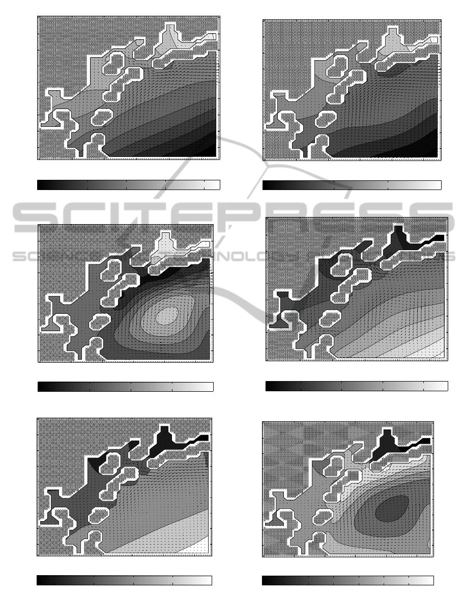
Fig. 5 at several time moments. Comparison with
Fig. 4 shows that a wind-driven flow occurs and is
then developing in the computational domain. Specif-
ically, as the simulation starts, the velocity field is
formed clockwise (Fig. 5, t = 0.2,0.4), in accordance
with the wind stress at small times (Fig. 4, top). Later,
at t = 0.5, the wind’s direction changes to anticlock-
wise due to the term sin2πt, which is reflected in the
numerical solution with a little time gap because of
the fluid’s inertia, especially in the open ocean far
from the coastline: while the coastal waters change
their flows at t ≈0.5−0.7, the large vortex in the open
bay begins rotating anticlockwise at t ≈ 0.8 (Fig. 5).
Finally, at t = 1 the entire velocity field is aligned in
accordance with the late-time wind stress (Fig. 4, bot-
tom).
SimulationofShallow-waterFlowsinComplexBay-likeDomains
29

λ
ϕ
Solution at t = 0.2 days
12.1 12.2 12.3 12.4 12.5 12.6
45.2
45.25
45.3
45.35
45.4
45.45
45.5
45.55
45.6
35.96 35.965 35.97 35.975 35.98
λ
ϕ
Solution at t = 0.4 days
12.1 12.2 12.3 12.4 12.5 12.6
45.2
45.25
45.3
45.35
45.4
45.45
45.5
45.55
45.6
35.845 35.85 35.855 35.86
λ
ϕ
Solution at t = 0.5 days
12.1 12.2 12.3 12.4 12.5 12.6
45.2
45.25
45.3
45.35
45.4
45.45
45.5
45.55
45.6
35.786 35.787 35.788 35.789 35.79
λ
ϕ
Solution at t = 0.7 days
12.1 12.2 12.3 12.4 12.5 12.6
45.2
45.25
45.3
45.35
45.4
45.45
45.5
45.55
45.6
35.74 35.745 35.75 35.755
λ
ϕ
Solution at t = 0.8 days
12.1 12.2 12.3 12.4 12.5 12.6
45.2
45.25
45.3
45.35
45.4
45.45
45.5
45.55
45.6
35.77 35.775 35.78 35.785 35.79
λ
ϕ
Solution at t = 1 days
12.1 12.2 12.3 12.4 12.5 12.6
45.2
45.25
45.3
45.35
45.4
45.45
45.5
45.55
45.6
35.887535.88835.888535.88935.889535.8935.8905
Figure 5: Problem 2, numerical solution at several time moments (the solution is reduced to a coarser grid ∆λ ≈ ∆ϕ ≈ 0.01
◦
for better visualisation; the fluid’s depth is shown by colour, while the velocity field is shown by arrows).
SIMULTECH2012-2ndInternationalConferenceonSimulationandModelingMethodologies,Technologiesand
Applications
30

4 CONCLUSIONS
A new fully discrete mass– and total-energy–
conserving finite difference model for the simulation
of shallow-water flows in bay-like domains with com-
plex boundaries was developed. Having taken the
SWEs written in the divergent form, we involved the
idea of operator splitting coupled with the Crank-
Nicolson approximation and constructed absolutely
stable second-order finite difference schemes that al-
low accurate simulation of shallow-water flows in
spherical domains of arbitrary shapes. An important
integral invariant of motion of the SWEs, the potential
enstrophy, proved to be bounded for an inviscid un-
forced fluid, oscillating in time within a narrow range.
Hence, the numerical solution is mathematically ac-
curate and provides physically adequate results. Due
to the method of splitting the developed model can
straightforwardly be implemented for distributed sim-
ulation of shallow-water flows on high-performance
parallel computers. Numerical experiments with a
simple inviscidunforced closed shallow-watersystem
and with a viscous open wind-driven shallow-water
model simulating a real situation nicely confirmed the
skills of the new method.
ACKNOWLEDGEMENTS
This research was partially supported by the grants
No. 14539 and No. 26073 of the National Sys-
tem of Researchers of Mexico (SNI), and is part of
the projects PAPIIT-UNAM IN104811 and PAPIME-
UNAM PE103311, Mexico.
REFERENCES
Agoshkov, V. I. and Saleri, F. (1996). Recent developments
in the numerical simulation of shallow water equa-
tions. part iii: Boundary conditions and finite element
approximations in the river flow calculations. Math.
Modelling, 8:3–24.
Arakawa, A. and Lamb, V. R. (1981). A potential enstrophy
and energy conserving scheme for the shallow-water
equation. Mon. Wea. Rev., 109:18–36.
Bouchut, F., Sommer, J. L., and Zeitlin, V. (2004). Frontal
geostrophic adjustment and nonlinear wave phenom-
ena in one-dimensional rotating shallow water. part
ii: High-resolution numerical simulations. J. Fluid
Mech., 514:35–63.
Heikes, R. and Randall, D. A. (1995). Numerical integra-
tion of the shallow-water equations on a twisted icosa-
hedral grid. part i: Basic design and results of tests.
Mon. Wea. Rev., 123:1862–1880.
Jirka, G. H. and Uijttewaal, W. S. J., editors (2004). Shallow
Flows, London. Taylor & Francis.
Kundu, P. K., Cohen, I. M., and Dowling, D. R. (2012).
Fluid Mecanics. Academic Press, 5th edition.
LeVeque, R. J. and George, D. L. (2007). High-resolution
finite volume methods for the shallow-water equations
with bathymetry and dry states. In Yeh, H., Liu,
P. L., and Synolakis, C. E., editors, Advanced Numeri-
cal Models for Simulating Tsunami Waves and Runup,
pages 43–73. World Scientific Publishing, Singapore.
Marchuk, G. I. (1982). Methods of Computational Mathe-
matics. Springer-Verlag, Berlin.
Oliger, J. and Sundstrom, A. (1978). Theoretical and prac-
tical aspects of some initial boundary value problems
in fluid dynamics. SIAM J. Appl. Anal., 35:419–446.
Pedlosky, J. (1987). Geophysical Fluid Dynamics. Springer,
2nd edition.
Press, W. H., Teukolsky, S. A., Vetterling, W. T., and Flan-
nery, B. P. (2007). Numerical Recipes: The Art of Sci-
entific Computing. Cambridge University Press, Cam-
bridge.
Ringler, T. D. and Randall, D. A. (2002). A potential en-
strophy and energy conserving numerical scheme for
solution of the shallow-water equations on a geodesic
grid. Mon. Wea. Rev., 130:1397–1410.
Sadourny, R. (1975). The dynamics of finite-difference
models of the shallow-water equations. J. Atmos. Sci.,
32:680–689.
Salmon, R. (2009). A shallow water model conserving en-
ergy and potential enstrophy in the presence of bound-
aries. J. Mar. Res., 67:1–36.
Shokin, Y. I. (1988). Completely conservative difference
schemes. In de Vahl Devis, G. and Fletcher, C., edi-
tors, Computational Fluid Dynamics, pages 135–155.
Elsevier, Amsterdam.
Simonnet, E., Ghil, M., Ide, K., Temam, R., and Wang, S.
(2003). Low-frequency variability in shallow-water
models of the wind-driven ocean circulation. part i:
Steady-state solution. J. Phys. Ocean., 33:712–728.
Skiba, Y. N. (1995). Total energy and mass conserving finite
difference schemes for the shallow-water equations.
Russ. Meteorol. Hydrology, 2:35–43.
Skiba, Y. N. and Filatov, D. M. (2008). Conservative arbi-
trary order finite difference schemes for shallow-water
flows. J. Comput. Appl. Math., 218:579–591.
Skiba, Y. N. and Filatov, D. M. (2009). Simulation of
soliton-like waves generated by topography with con-
servative fully discrete shallow-water arbitrary-order
schemes. Internat. J. Numer. Methods Heat Fluid
Flow, 19:982–1007.
Vol’tsynger, N. E. and Pyaskovskiy, R. V. (1977). Theory of
Shallow Water. Gidrometeoizdat, St. Petersburg.
Vreugdenhil, C. B. (1994). Numerical Methods for
Shallow-Water Flow. Kluwer Academic, Dordrecht.
SimulationofShallow-waterFlowsinComplexBay-likeDomains
31