
Unified Algorithm to Improve Reinforcement Learning
in Dynamic Environments
An Instance-based Approach
Richardson Ribeiro
1
, F
´
abio Favarim
1
, Marco A. C. Barbosa
1
,
Andr
´
e Pinz Borges
2
, Osmar Betazzi Dordal
2
, Alessandro L. Koerich
2
and Fabr
´
ıcio Enembreck
2
1
Graduate Program in Computer Engineering, Federal Technological University of Paran
´
a, Pato Branco, Paran
´
a, Brazil
2
Post-Graduate Program in Computer Science, Pontificial Catholical University of Paran
´
a, Curitiba, Paran
´
a, Brazil
Keywords:
Intelligent Agents, Reinforcement Learning, Dynamic Environments.
Abstract:
This paper presents an approach for speeding up the convergence of adaptive intelligent agents using reinforce-
ment learning algorithms. Speeding up the learning of an intelligent agent is a complex task since the choice
of inadequate updating techniques may cause delays in the learning process or even induce an unexpected
acceleration that causes the agent to converge to a non-satisfactory policy. We have developed a technique for
estimating policies which combines instance-based learning and reinforcement learning algorithms in Marko-
vian environments. Experimental results in dynamic environments of different dimensions have shown that the
proposed technique is able to speed up the convergence of the agents while achieving optimal action policies,
avoiding problems of classical reinforcement learning approaches.
1 INTRODUCTION
Markov Decision Processes (MDP) are a popular
framework for sequential decision-making for single
agents, when agents’ actions have stochastic effect on
the environment state and need to learn how to ex-
ecute sequential actions. Adaptive intelligent agents
emerge as an alternative to cope with several com-
plex problems including control, optimization, plan-
ning, manufacturing and so on. A particular case is
an environment where events and changes in policy
may occur continuously (i.e., dynamic environment).
A way of addressing such a problem is to use Rein-
forcement Learning (RL) algorithms, which are often
used to explore a very large space of policies in an
unknown environment by trial and error. It has been
shown that RL algorithms, such as the Q-Learning al-
gorithm (Watkins and Dayan, 1992), converge to opti-
mal policies when a large number of trials are carried
out in stationary environments (Ribeiro, 1999).
Several works using RL algorithms and adaptive
agents in different applications can be found in the
literature (Tesauro, 1995; Strehl et al., 2009; Zhang
et al., 2010). However, one of the main drawbacks of
RL algorithms is the rate of convergence which can
be too slow for many real-world problems, e.g.
traffic environments, sensor networks, supply chain
management and so forth. In such problems, there is
no guarantee that RL algorithms will converge, since
they were originally developed and applied to static
problems, where the objective function is unchanged
over time. However, there are few real-world prob-
lems that are static, i.e. problems in which changes
in priorities for resources do not occur, goals do not
change, or where there are tasks that are no longer
needed. Where changes are needed through time, the
environment is dynamic.
In such environments, several approaches for
achieving rapid convergence to an optimal pol-
icy have been proposed in recent years (Price and
Boutilier, 2003; Bianchi et al., 2004; Comanici and
Precup, 2010; Banerjee and Kraemer, 2010). They
are based mainly on the exploration of the state-action
space, leading to a long learning process and requir-
ing great computational effort.
To improve convergence rate, we have developed
an instance-based reinforcement learning algorithm
coupled with conventional exploration strategies such
as the ε-greedy (Sutton and Barto, 1998). The algo-
rithm is better able to estimate rewards, and to gen-
erate new action policies, than conventional RL algo-
rithms. An action policy is a function mapping states
229
Ribeiro R., Favarim F., A. C. Barbosa M., Pinz Borges A., Betazzi Dordal O., L. Koerich A. and Enembreck F..
Unified Algorithm to Improve Reinforcement Learning in Dynamic Environments - An Instance-based Approach.
DOI: 10.5220/0004000002290238
In Proceedings of the 14th International Conference on Enterprise Information Systems (ICEIS-2012), pages 229-238
ISBN: 978-989-8565-10-5
Copyright
c
2012 SCITEPRESS (Science and Technology Publications, Lda.)

to actions by estimating a probability that a state s
0
can be reached after taking action a in state s.
In MDP, algorithms attempt to compute a policy
such that the expected long-term reward is maximized
by interacting with an environment (Ribeiro, 1999).
The approach updates into state-action space the re-
wards of unsatisfactory policies generated by the RL
algorithm. States with similar features are given sim-
ilar rewards; rewards are anticipated and the number
of iterations in the Q-learning algorithm is decreased.
In this paper we show that, even in partially-
known and dynamic environments, it is possible to
achieve a policy close to the optimal very quickly. To
measure the quality of our approach we use a station-
ary policy computed previously, comparing the return
from our algorithm with that from the stationary pol-
icy, as in (Ribeiro et al., 2006).
This article is organized as follows: Section 2 in-
troduces the RL principles and the usage of heuristics
to discover action policies. The technique proposed
for dynamic environments is presented in Section 3
where we also discuss the Q-Learning algorithm and
the k-Nearest Neighbor (k-NN) algorithm. Section
4 gives experimental results obtained using the pro-
posed technique. In the final section, some conclu-
sions are stated and some perspectives for future work
are discussed.
2 BACKGROUND AND
NOTATION
Many real-life problems such as games (Jordan et al.,
2010; Amato and Shani, 2010), robotics (Spaan and
Melo, 2008), traffic light control (Mohammadian,
2006; Le and Cai, 2010) or air traffic (Sislak et al.,
2008; Dimitrakiev et al., 2010), occur in dynamic en-
vironments. Agents that interact in this kind of envi-
ronment need techniques to help them, e.g., to reach
some goal, to solve a problem or to improve perfor-
mance. However because individual circumstances
are so diverse, it is difficult to propose a generic ap-
proach (heuristics) that can be used to deal with every
kind of problem. Environment is the world in which
an agent operates.
A dynamic environment consists of changing sur-
roundings in which the agent navigates. It changes
over time independent of agent actions. Thus, un-
like the static case, the agent must adapt to new sit-
uations and overcome possibly unpredictable obsta-
cles (Firby, 1989; Pelta et al., 2009). Traditional plan-
ning systems have presented problems when dealing
with dynamic environments. In particular, issues such
as truth maintenance in the agent’s symbolic world
model, and replanning in response to changes in the
environment, must be addressed.
Predicting the behavior (i.e., actions) of an adap-
tive agent in dynamic environments is a complex
task. The actions chosen by the agent are often unex-
pected, which makes it difficult to choose a good tech-
nique (or heuristic) to improve agent performance. A
heuristic can be defined as a method that improves
the efficiency in searching a problem solution, adding
knowledge about the problem to an algorithm.
Before discussing related work, we introduce the
MDP which is used to describe our domain. A MDP
is a tuple (S,A,∂
a
s,s
0
,R
a
s,s
0
,γ) where S is a discrete set
of environment states that can be composed by a se-
quence of state variables < x
1
,x
2
,...,x
y
>. An episode
is a sequence of actions a ∈ A that leads the agent
from a state s to s
0
. ∂
a
s,s
0
is a function defining the
probability that the agent arrives in state s
0
when an
action a is applied in state s. Similarly, R
a
s,s
0
is the re-
ward received whenever the transition ∂
a
s,s
0
occurs and
γ ∈ {0...1} is a discount rate parameter.
A RL agent must learn a policy Q : S → A that
maximizes its expected cumulative reward (Watkins
and Dayan, 1992), where Q(s, a) is the probability of
selecting action a from state s. Such a policy, denoted
as Q
∗
, must satisfy Bellman’s equation (Sutton and
Barto, 1998) for each state s ∈ S (Equation 1).
Q(s,a) ← R(s, a) + γ
∑
s
0
∂(s,a,s
0
) × max Q(s
0
,a) (1)
where γ weights the value of future rewards and
Q(s,a) is the expected cumulative reward given for
executing an action a in state s. To reach an optimal
policy (Q
∗
), a RL algorithm must iteratively explore
the space S × A updating the cumulative rewards and
storing such values in a table
ˆ
Q.
In the Q-learning algorithm proposed by Watkins
(Watkins and Dayan, 1992), the task of an agent is to
learn a mapping from environment states to actions
so as to maximize a numerical reward signal. The
algorithm approaches convergence to Q
∗
by applying
an update rule (Equations (2)(3)) after a time step t:
v ← γ max Q
t
(s
t+1
,a
t+1
) − Q
t
(s
t
,a
t
) (2)
Q
t+1
(s
t
,a
t
) ← Q
t
(s
t
,a
t
) + α[R(s
t
,a
t
) + v] (3)
where V is the utility value to perform an action a in
state s and α ∈ {0, 1} is the learning rate.
In dynamic environments such as traffic jams, it
is helpful to use strategies like ε-greedy exploration
(Sutton and Barto, 1998) where the agent selects an
action with the greatest Q value with probability 1−ε.
ICEIS2012-14thInternationalConferenceonEnterpriseInformationSystems
230

In some Q-Learning experiments, we have found that
the agent does not always converge during training
(see Section 4). To overcome this problem we have
used a well known Q-Learning property: actions can
be chosen using an exploration strategy. A very com-
mon strategy is random exploration, where an action
is randomly chosen with probability ε and the state
transition is given by Equation 4.
Q(s) =
maxQ(s,a) ,i f q > ε
a
random
,otherwise
(4)
where q is a random value with uniform probabil-
ity in [0, 1] and ε ∈ [0, 1] is a parameter that defines
the exploration trade-off. The greater the value of ε,
the smaller is the probability of a random choice, and
a
random
is a random action selected among the possi-
ble actions in state s.
Several authors have shown that matching some
techniques with heuristics can improve the perfor-
mance of agents, and that traditional techniques, such
as ε-greedy, yield interesting results (Drummond,
2002; Price and Boutilier, 2003; Bianchi et al., 2004).
Bianchi (Bianchi et al., 2004) proposed a new class
of algorithms aimed at speeding up the learning of
good action policies. An RL algorithm uses a heuris-
tic function to force the agent to choose actions during
the learning process. The technique is used only for
choosing the action to be taken, while not affecting
the operation of the algorithm or modifying its prop-
erties.
Butz (Butz, 2002) proposes the combination of an
online model learner with a state value learner in a
MDP. The model learner learns a predictive model
that approximates the state transition function of the
MDP in a compact, generalized form. State values are
evaluated by means of the evolving predictive model
representation. In combination, the actual choice of
action depends on anticipating state values given by
the predictive model. It is shown that this combina-
tion can be applied to increase further the learning of
an optimal policy
Bianchi et al. (Bianchi et al., 2008) improved ac-
tion selection for online policy learning in robotic sce-
narios combining RL algorithms with heuristic func-
tions. The heuristics can be used to select appropri-
ate actions, so as to guide exploration of the state-
action space during the learning process, which can
be directed towards useful regions of the state-action
space, improving the learner behavior, even at initial
stages of the learning process.
In this paper we propose going further in the use
of exploration strategies to achieve a policy closer to
the Q
∗
. To do this we have used policy estimation
techniques based on an instance learning, such as the
k-Nearest Neighbors (k-NN) algorithm. We have ob-
served that is possible to reuse previous states, elimi-
nating the need of a prior heuristic.
3 K-NR: INSTANCE-BASED
REINFORCEMENT LEARNING
APPROACH
In RL, learning takes place through a direct interac-
tion of the algorithm with the agent and the environ-
ment. Unfortunately, the convergence of the RL al-
gorithms can only be reached after an exhaustive ex-
ploration of the state-action space, which usually con-
verges very slowly. However, the convergence of the
RL algorithm may be accelerated through the use of
strategies dedicated to guiding the search in the state-
action space.
The proposed approach, named k-Nearest Rein-
forcement (k-NR), has been developed from the ob-
servation that algorithms based on different learning
paradigms may be complementary to discover action
policies (Kittler et al., 1998). The information gath-
ered during the learning process of an agent with the
Q-Learning algorithm is the input for the k-NR. The
reward values are calculated with an instance-based
learning algorithm. This algorithm is able to accumu-
late the learned values until a suitable action policy is
reached.
To analyze the convergence of the agent with the
k-NR algorithm, we assume a generative model gov-
erning the optimal policy. With such a model it is pos-
sible to evaluate the learning table generated by the
Q-Learning algorithm. To do this, an agent is inserted
into a partially known environment with the following
features:
1. Q-Learning Algorithm: learning rate (α), dis-
count factor (γ) and reward (r);
2. Environment E: the environment consists of a
state space where there is an initial state (s
initial
), a
goal state (s
goal
) and a set of actions A={↑, ↓, →,
←}, where ↑, ↓, →, ← mean respectively east,
south, north and west (Figure 1).
A state s is an ordered pair (x, y) with positional
coordinates on the axis X and Y respectively. In other
words, the set of states S represents a discrete city
map. A status function st : S → ST maps states and
traffic situations where ST = {-0.1, -0.2, -0.3, -0.4
, -1.0, 1.0 )}, where -0.1, -0.2, -0.3, -0.4, -1.0 and
1.0 mean respectively free, low jam, jam or unknown,
high jam, blocked, and goal. After each move (tran-
sition) from state s to s
0
the agent knows whether its
UnifiedAlgorithmtoImproveReinforcementLearninginDynamicEnvironments-AnInstance-basedApproach
231
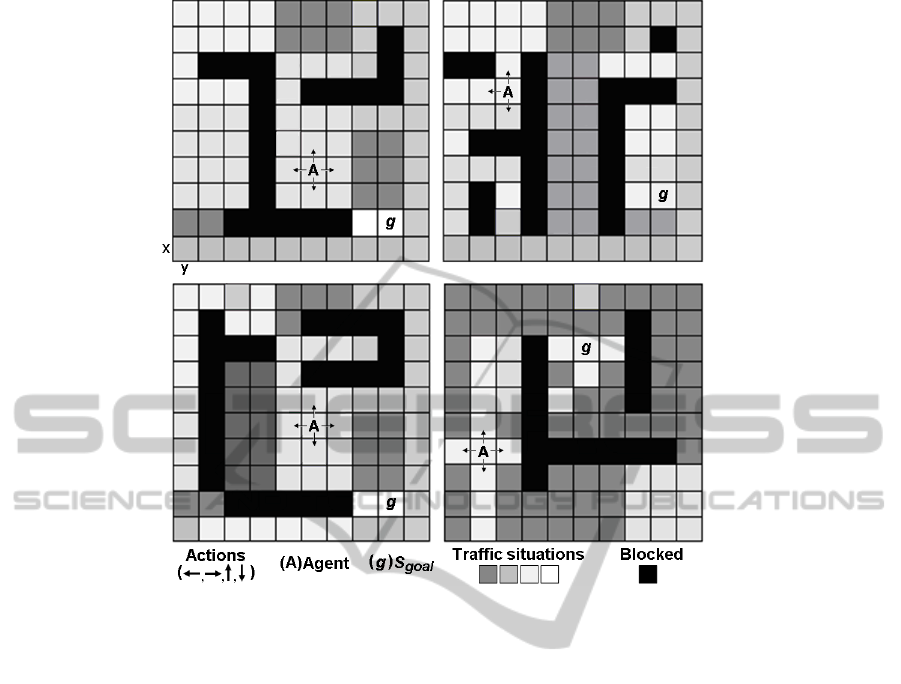
Figure 1: Environment: An agent is placed at random positions in the grid, having a visual field depth of 1.
action is positive or negative through the rewards at-
tributed by the environment. Thus, the reward for a
transition ∂
a
s,s
0
is st(s
0
) and Equations (2) (3) is used as
update function. In other words, the agent will know
if its action has been positive if, having found itself
in a state with traffic jam, its action has led to a state
where the traffic jam is less severe. However, if the
action leads the agent to a more congested status then
it receives a negative reward.
The pseudocode to estimate the values for the
learning parameters for the Q-Learning using the k-
NR is presented in Algorithm 1. The following defi-
nitions parameters are used in such an algorithm:
• a set S = {s
1
,.. . , s
m
} of states;
• an instant discrete steps step = 1, 2, 3, ...,n;
• a time window T
x
that represents the learning time
(cycle(x) of steps);
• a set A = {a
1
,.. . , a
m
} of actions, where each ac-
tion is executable in a step n;
• a status function st : S → ST where ST =
{−1,−0.4,−0.3, −0.2, −0.1};
• learning parameters: α=0.2 and γ=0.9;
• a learning table QT : (S × A) → R used to store
the accumulative rewards calculated with the Q-
Learning algorithm;
• a learning table kT : (S × A) → R used to store the
reward values estimated with the k-NN;
• #changes is the number of changes in the environ-
ment.
3.1 k-NN and k-NR
The instance-based learning paradigm determines the
hypothesis directly from training instances. Thus, the
k-NN algorithm saves training instances in the mem-
ory as points in an n-dimensional space, defined by
the n attributes which describe them (Aha et al., 1991;
Galvn et al., 2011). When a new instance must be
classified, the most frequent class among the k near-
est neighbors is chosen. In this paper the k-NN algo-
rithm is used to generate intermediate policies which
speed up the convergence of RL algorithms. Such an
algorithm receives as input a set of instances gener-
ated from an action policy during the learning stage
of the Q-Learning. For each environment state, four
instances are generated (one for each action) and they
represent the values learned by the agent. Each train-
ing instance has the following attributes:
ICEIS2012-14thInternationalConferenceonEnterpriseInformationSystems
232

1. attributes for the representation of the state in the
way of the expected rewards for the actions: north
(N), south (S), east (E) and west (W);
2. an action and;
3. reward for this action.
Table 1 shows some examples of training in-
stances.
Algorithm 2 shows that the instances are com-
puted to a new table, denoted as kT , which stores the
values generated by the k-NR with the k-NN. Such
values represent the sum of the rewards received with
the interaction with the environment. Rewards are
computed using Equation 6 which calculates the sim-
Algorithm 1: Policy estimation with k-NR.
Require: Learning Table: QT (s,a);
kT (s,a); S={s
1
, ..., s
m
}; A={a
1
, ..., a
m
}
st: S → ST;
Time window T
x
;
Environment E;
Ensure:
1. for all s ∈ S do
2. for all a ∈ A do
3. QT (s, a) ← 0;
4. kT (s,a) ← 0;
5. end for
6. end for
7. while not stop condition() do
8. CHOOSE s ∈ S, a ∈ A
9. Update rule:
10. Q
t+1
(s
t
,a
t
) ← Q
t
(s
t
,a
t
)+α[R(s
t
,a
t
)+v]
where,
11. v ← γ max Q
t
(s
t+1
,a
t+1
)−Q
t
(s
t
,a
t
)
12. step ← step + 1;
13. if step < T
x
then
14. GOTO{8};
15. end if
16. if changes are supposed to occur then
17. for I ← 1 to #changes do
18. Choose s ∈ S
19. st(s) ← a new status st ∈ ST;
20. end for
21. Otherwise continue()
22. end if
23. k-NR(T
x
,s,a); // Algorithm 2
24. for s ∈ S do
25. for a ∈ A do
26. QT (s, a) ← kT (s,a)
27. end for
28. end for
29. end while
30. return (.,.);
Algorithm 2: k-NR(T
x
,s, a).
1: for all s ∈ S and s 6= s
goal
do
2: costQT ← cost(s, s
goal
, QT)
3: costQ
∗
← cost(s, s
goal
, Q
∗
)
4: if costQT
s
6= costQ∗
s
then
5:
kT (s,a) ←
∑
k
i=1
HQ
i
(.,.)
k
(5)
6: end if
7: end for
8: return (kT (s,a))
ilarity between two training instances
~
s
i
and
~
s
m
.
f (
~
s
i
,
~
s
m
) =
∑
x
x=1
(s
i
x
× s
m
x
)
∑
x
x=1
s
2
i
x
×
∑
x
x=1
s
2
m
x
(6)
The cost function (Equation 7) calculates the cost
for an episode (path from a current state s to the state
s
goal
based on the current policy).
cost(s,s
goal
) =
s
goal
∑
s∈S
0.1 +
s
goal
∑
s∈S
st(s) (7)
Equation 5 used in Algorithm 2 shows how the
k-NN algorithm can be used to generate the arrange-
ments of training instances: here, kT (s, a) is the es-
timated reward value for a given state s and action a,
k is the number of nearest neighbors, and HQ
i
(.,.) is
the i-th existing nearest neighbor in the set of training
instances generated from QT (s, a).
Using the k-NR, the values learned by the Q-
Learning are stored in the kT table. This contains the
best values generated by the Q-Learning and the val-
ues that have been estimated by the k-NR.
We have evaluated different ways of generating
the arrangements of instances for the k-NN algorithm
with the aim of finding the best training sets. First,
we used the full arrangement of instances generated
throughout runtime. Second, instances generated in-
side n time windows were selected, where A
[T (n)]
de-
notes an arrangement of T (n) windows. In this core,
each window generates a new arrangement and previ-
ously instances are discarded. We have also evaluated
the efficiency rate considering only the arrangement
given by the last window A
[T (last)]
. Finally, we have
evaluated the efficiency rate of the agent using the
last arrangement calculated by the k-NN algorithm -
A
[T (last),T (k−NN)]
. The results on these different con-
figurations for generating instances are shown in Sec-
tion 4.
UnifiedAlgorithmtoImproveReinforcementLearninginDynamicEnvironments-AnInstance-basedApproach
233
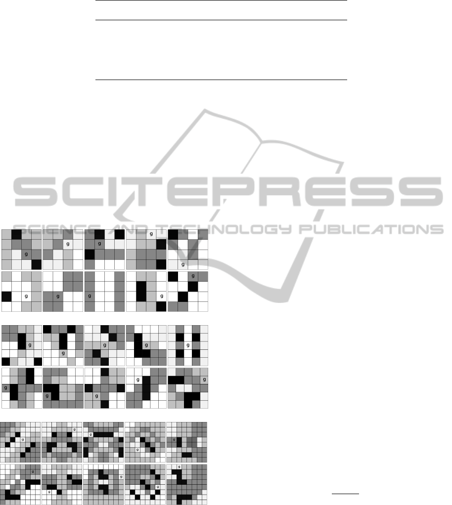
Table 1: Training instances.
State Reward Reward Reward Reward Action Reward
(x,y) (N) (S) (E) (W) Chosen Action
(2,3) -0.875 -0.967 0.382 -0.615 (N) -0.875
(2,3) -0.875 -0.968 0.382 -0.615 (S) -0.968
(2,3) -0.875 -0.968 0.382 -0.615 (W) 0.382
(2,3) -0.875 -0.968 0.382 -0.615 (E) -0.615
(1,2) -0.144 1.655 -0.933 0.350 (N) -0.144
.. . .. . .. . .. . .. . .. . .. .
4 EXPERIMENTAL RESULTS
In this section we present the main results obtained
from using the k-NR and Q-Learning algorithms. The
experiments were carried out in dynamic environ-
ments with three different sizes as shown in Figure 2:
16 (4×4), 25 (5×5) and 64 (8×8) states. Note that a
number of states S can generate a long solution space,
in which the number of possible policy is |A||
s
|.
(a)
(b)
(c)
Figure 2: Simulated environments: (a) 16-state, (b) 25-
state, (c) 64-state.
For each size of environment, ten different config-
urations were arbitrarily generated to simulate real-
world scenarios. The learning process was repeated
twenty times for each environment configuration to
evaluate the variations that can arise from the agent’s
actions which are autonomous and stochastic. The re-
sults presented in this section for each environment
size (16, 25, and 64) are therefore average values over
twenty runs. The results do not improve significantly
when more scenarios are used (≈2.15%). The effi-
ciency of the k-NR and Q-Learning algorithms (Y axis
in figures) takes into account the number of successful
outcomes of a policy in a cycle of steps. We evaluated
the agent’s behavior in two situations:
1. ]percent of changes (10, 20, 30) in environment
for a window T
x
=100. In 64-state environments
the changes were inserted after each 1000 steps
(T
x
=1000) because in dynamic environments such
large environments require many steps to reach a
good intermediary policy.
2. ]percent of changes in environment after the agent
finds its best action policy. In this case, we use the
full arrangement of learning instances A
[T
x
]
, be-
cause it gave the best results.
The changes were simulated considering real traf-
fic conditions such as: different levels of traffic jams,
partial blocking and free traffic for vehicle flowing.
We also allowed for the possibility that unpredictable
factors may change traffic behavior, such as accidents,
route changing or roadway policy, collisions in traffic
lights or intersections, and so on. Changes in the envi-
ronment were made as follows: for every T
x
window,
the status of a number of positions is altered random.
Equation 8 is used to calculate the number of altered
states (]changes) in T
x
.
]changes
(T
x
)
=
]states
100
× ]percent (8)
We observed in initial experiments, that even with
a low change rate in the environment, the agent with
Q-Learning has trouble converging without the sup-
port of exploration strategies.
To solve this problem, we used the Q-Learning to-
gether with the ε-greedy strategy, which allows the
agent to explore states with low rewards. With such a
strategy, the agent starts to re-explore the states that
ICEIS2012-14thInternationalConferenceonEnterpriseInformationSystems
234
underwent changes in their status. More detail of
the ε-greedy strategy in others scenarios are given in
(Ribeiro et al., 2006). It can be seen from this ex-
periment that the presence of changed states in an ac-
tion policy may decrease the agent’s convergence sig-
nificantly. Thus, the reward values that would lead
the agent to states with positive rewards can cause
the agent to search over states with negative rewards,
causing errors. In the next experiments we therefore
introduce the k-NR.
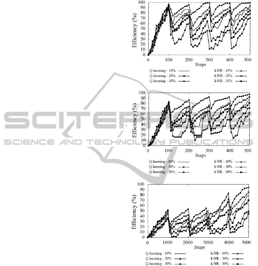
4.1 k-NR Evaluation
We used the k-NR to optimize the performance of Q-
Learning. The technique was applied only to the envi-
ronment states where changes occur. Thus, the agent
modifies its learning and converges more rapidly to a
good action policy. Figure 3 shows how this mod-
ification in the heuristic affects convergence of Q-
Learning. However using k-NR, the agent rapidly
converges to a good policy, because it uses reward val-
ues that were not altered when the environment was
changed.
It is seen that the proposed approach may acceler-
ate convergence of the RL algorithms, while decreas-
ing the noise rate during the learning process. More-
over, in dynamic environments the aim is to find al-
ternatives which decrease the number of steps that the
agent takes until it starts to converge again. The k-NR
algorithm causes the agent to find new action policies,
for the states that have had their status altered by the
reward values of unaltered neighbor states. In some
situations, the agent may continue to convergeeven
after a change of the environment. This happens be-
cause some states have poor reward values (values
that are either too high or too low) as a consequence
of too few visits, or too many. Therefore, such states
must be altered by giving them more appropriate re-
ward values.
To observe the behavior of the agent in other situ-
ations, changes were introduced into the environment
only after the agent finds its near-optimal policy (a
policy is optimal when the agent knows the best ac-
tions). The aim is to analyze the agent’s performance
when an optimal or near-optimal policy has been dis-
covered, and to observe the agent’s capacity then to
adapt itself to a modified environment.
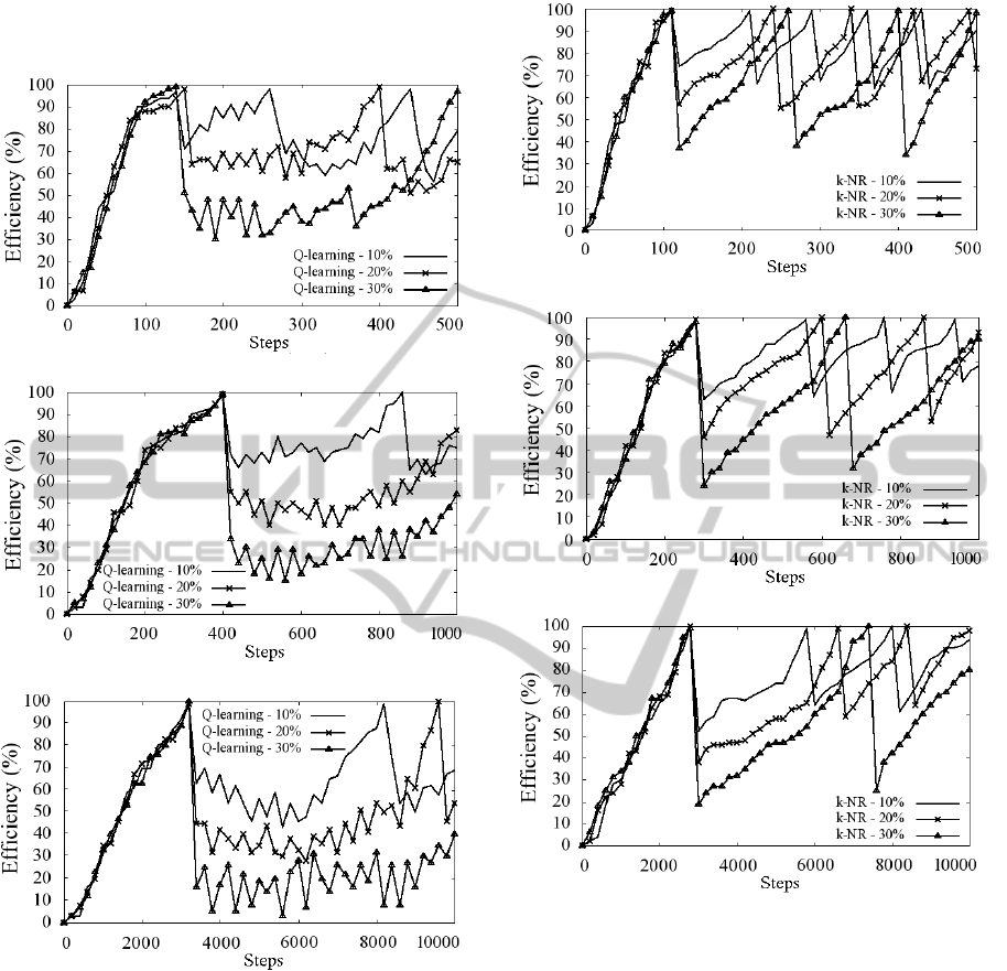
Enembreck et al. (Enembreck et al., 2007) have
shown that this is a good way to observe the behavior
of an adaptive agent. We have analyzed the agent’s
adaptation with the k-NR and Q-Learning algorithms.
The Q-Learning presents a period of divergence (after
some changes were generated), usually a decreasing
performance (Figure 4). However, after a reasonable
(a)
(b)
(c)
Figure 3: Performance of the K-NR and Q-Learning algo-
rithms in a: (a) 16-state environment, (b) 25-state environ-
ment, (c) 64-state environment.
number of steps, it is seen that there is again con-
vergence to a better policy, as happens when learn-
ing begins and performance improves. The decreas-
ing performance occurs because Q-Learning needs to
re-explore all the state space, re-visiting states with
low rewards to accumulate better values for the future.
The ε-greedy strategy helps the agent by introducing
random actions so that local maxima are avoided. For
UnifiedAlgorithmtoImproveReinforcementLearninginDynamicEnvironments-AnInstance-basedApproach
235
example, a blocked state that changed to low jam must
have negative rewards and would no longer be visited.
(a)
(b)
(c)
Figure 4: Agent adaptation using the Q-Learning in a: (a)
16-state environment, (b) 25-state environment, (c) 64-state
environment.
We used the k-NR algorithm with heuristic to op-
timize agent performance with the methodology dis-
cussed in Section 2, which uses instance-based learn-
ing in an attempt to solve the problem described in the
previous subsection. The heuristic has been applied
only to the environment states where changes occur.
Thus, the heuristic usually caused the agent to mod-
ify its learning and converge more rapidly to a good
action policy.
Figure 4 also shows that the Q-Learning does not
show uniform convergence when compared with k-
(a)
(b)
(c)
Figure 5: Agent adaptation using the k-NR in a: (a) 16-state
environment, (b) 25-state environment, (c) 64-state environ-
ment.
NR (Figure 5). This occurs because the k-NR algo-
rithm uses instance-based learning, giving superior
performance and speeding up its convergence. The
k-NR is able to accelerate the convergence because
the states that have had their status altered were esti-
mated from similar situations observed in the past, so
that states with similar features have similar rewards.
Table 2 shows the number of steps needed for the
agent to re-find its best action policy. It is seen that
k-NR performs better than standard Q-Learning. In
16-state environments, the agent finds its best policy
of actions with 150 steps using the Q-Learning algo-
rithm and 110 steps with k-NR. After changing the en-
ICEIS2012-14thInternationalConferenceonEnterpriseInformationSystems
236

Table 2: Number of steps needed for the agent to find its best policy after changes.
Before changes After changes
10% 20% 30%
] states Q k Q k Q k Q k
16 150 110 130 90 240 140 350 150
25 400 280 440 290 1130 320 2140 380
64 3,430 2,830 5,450 2,950 6,100 3,850 13,900 4,640
vironment with 10%, 20% and 30% the k-NR needed
47% fewer steps on average before it once again finds
a policy leading to convergence. For 25-state environ-
ments the agent finds its best action policy in approx-
imately 400 steps using Q-Learning, and in 280 steps
with k-NR. In this environment, k-NR uses an average
of 30% fewer steps than Q-Learning, after alteration
of the environment. For 64-state environments, the
agent needed an average of 3,430 steps to find its best
action policy with Q-Learning and 2,830 with k-NR.
The k-NR used in average 18% fewer steps than Q-
Learning after environmental change. It is seen that
k-NR is more robust in situations where the reward
values vary unpredictably. This happens because the
k-NN algorithm is less sensitive to noisy data.
5 DISCUSSION AND
CONCLUSIONS
This paper has introduced a technique for speeding up
convergence of a policy defined in dynamic environ-
ments. This is possible through the use of instance-
based learning algorithms. Results obtained when
the approach is used show that RL algorithms us-
ing instance-based learning can improve their per-
formance in environments with configurations that
change. From the experiments, it was concluded that
the algorithm is robust in partially-known and com-
plex dynamic environments, and can help to deter-
mine optimum actions. Combining algorithms from
different paradigms is an interesting approach for the
generation of good action policies. Experiments made
with the k-NR algorithm show that although compu-
tational costs are higher, the results are encouraging
because it is able to estimate values and find solutions
that support the standard Q-Learning algorithm.
We also observed benefits related to other works
using heuristic approaches. For instance, Bianchi et
al. (Bianchi et al., 2004) proposes a heuristic for
RL algorithms that show a significantly better perfor-
mance (40%) than the original algorithms. Pegoraro
et al. (Pegoraro et al., 2001) use a strategy that speeds
up the convergence of the RL algorithms by 36%,
thus reducing the number of iterations compared with
traditional RL algorithms. Although the results ob-
tained with the new technique are satisfactory, addi-
tional experiments are needed to answer some ques-
tions raised. For example, a multi-agent architecture
could be used to explore states placed further from the
goal-state and in which the state rewards are smaller.
Some of these strategies are found in Ribeiro et al.
(Ribeiro et al., 2008; Ribeiro et al., 2011). We also
intend to use more than one agent to analyze situ-
ations as: i) sharing with other agents the learning
of the best-performing one; ii) sharing learning val-
ues among all the agents simultaneously; iii) sharing
learning values among the best agents only; iv) shar-
ing learning values only when the agent reaches the
goal-state, in which its learning table would be uni-
fied with the tables of the others. Another possibility
is to evaluate the algorithm in higher-dimension en-
vironments, that are also subject to greater variations.
These possibilities will be explored in future research.
REFERENCES
Aha, D. W., Kibler, D., and Albert, M. K. (1991).
Instance-based learning algorithms. Machine Learn-
ing, 6(1):37–66.
Amato, C. and Shani, G. (2010). High-level reinforce-
ment learning in strategy games. In Proc. 9th Inter-
national Conference on Autonomous Agents and Mul-
tiagent Systems (AAMAS’10), pages 75–82.
Banerjee, B. and Kraemer, L. (2010). Action discovery
for reinforcement learning. In Proc. 9th International
Conference on Autonomous Agents and Multiagent
Systems (AAMAS’10), pages 1585–1586.
Bianchi, R. A. C., Ribeiro, C. H. C., and Costa, A. H. R.
(2004). Heuristically accelerated q-learning: A new
approach to speed up reinforcement learning. In Proc.
XVII Brazilian Symposium on Artificial Intelligence,
pages 245–254, So Luis, Brazil.
Bianchi, R. A. C., Ribeiro, C. H. C., and Costa, A. H. R.
(2008). Accelerating autonomous learning by using
heuristic selection of actions. Journal of Heuristics,
14:135–168.
Butz, M. (2002). State value learning with an anticipatory
learning classifier system in a markov decision pro-
cess. Technical report, Illinois Genetic Algorithms
Laboratory.
UnifiedAlgorithmtoImproveReinforcementLearninginDynamicEnvironments-AnInstance-basedApproach
237

Comanici, G. and Precup, D. (2010). Optimal policy
switching algorithms for reinforcement learning. In
Proc. 9th International Conference on Autonomous
Agents and Multiagent Systems (AAMAS’10), pages
709–714.
Dimitrakiev, D., Nikolova, N., and Tenekedjiev, K. (2010).
Simulation and discrete event optimization for auto-
mated decisions for in-queue flights. Int. Journal of
Intelligent Systems, 25(28):460–487.
Drummond, C. (2002). Accelerating reinforcement learn-
ing by composing solutions of automatically identified
subtask. Journal of Artificial Intelligence Research,
16:59–104.
Enembreck, F., Avila, B. C., Scalabrini, E. E., and Barthes,
J. P. A. (2007). Learning drifting negotiations. Applied
Artificial Intelligence, 21:861–881.
Firby, R. J. (1989). Adaptive Execution in Complex Dy-
namic Worlds. PhD thesis, Yale University.
Galvn, I., Valls, J., Garca, M., and Isasi, P. (2011). A lazy
learning approach for building classification models.
Int. Journal of Intelligent Systems, 26(8):773–786.
Jordan, P. R., Schvartzman, L. J., and Wellman, M. P.
(2010). Strategy exploration in empirical games. In
Proc. 9th International Conference on Autonomous
Agents and Multiagent Systems (AAMAS’10), v. 1,
pages 1131–1138, Toronto, Canada.
Kittler, J., Hatef, M., Duin, R. P. W., and Matas, J. (1998).
On combining classifiers. IEEE Transactions on Pat-
tern Analysis and Machine Intelligence, 20(3):226–
239.
Le, T. and Cai, C. (2010). A new feature for approx-
imate dynamic programming traffic light controller.
In Proc. 2th International Workshop on Computa-
tional Transportation Science (IWCTS’10), pages 29–
34, San Jose, CA, U.S.A.
Mohammadian, M. (2006). Multi-agents systems for intel-
ligent control of traffic signals. In Proc. International
Conference on Computational Inteligence for Mod-
elling Control and Automation and Int. Conf. on Intel-
ligent Agents Web Technologies and Int. Commerce,
page 270, Sydney, Australia.
Pegoraro, R., Costa, A. H. R., and Ribeiro, C. H. C. (2001).
Experience generalization for multi-agent reinforce-
ment learning. In Proc. XXI International Conference
of the Chilean Computer Science Society, pages 233–
239, Punta Arenas, Chile.
Pelta, D., Cruz, C., and Gonzlez, J. (2009). A study on
diversity and cooperation in a multiagent strategy for
dynamic optimization problems. Int. Journal of Intel-
ligent Systems, 24(18):844–861.
Price, B. and Boutilier, C. (2003). Accelerating reinforce-
ment learning through implicit imitation. Journal of
Artificial Intelligence Research, 19:569–629.
Ribeiro, C. H. C. (1999). A tutorial on reinforcement learn-
ing techniques. In Proc. Int. Joint Conference on Neu-
ral Networks, pages 59–61, Washington, USA.
Ribeiro, R., Borges, A. P., and Enembreck, F. (2008). Inter-
action models for multiagent reinforcement learning.
In Proc. 2008 International Conferences on Compu-
tational Intelligence for Modelling, Control and Au-
tomation; Intelligent Agents, Web Technologies and
Internet Commerce; and Innovation in Software En-
gineering, pages 464–469, Vienna, Austria.
Ribeiro, R., Borges, A. P., Ronszcka, A. F., Scalabrin, E.,
Avila, B. C., and Enembreck, F. (2011). Combinando
modelos de interao para melhorar a coordenao em sis-
temas multiagente. Revista de Informtica Terica e
Aplicada, 18:133–157.
Ribeiro, R., Enembreck, F., and Koerich, A. L. (2006).
A hybrid learning strategy for discovery of policies
of action. In Proc. International Joint Conference
X Ibero-American Artificial Intelligence Conference
and XVIII Brazilian Artificial Intelligence Symposium,
pages 268–277, Ribeiro Preto, Brazil.
Sislak, D., Samek, J., and Pechoucek, M. (2008). Decentral-
ized algorithms for collision avoidance in airspace. In
Proc. 7th International Conference on AAMAS, pages
543–550, Estoril, Portugal.
Spaan, M. T. J. and Melo, F. S. (2008). Interaction-driven
markov games for decentralized multiagent planning
under uncertainty. In Proc. 7th International Confer-
ence on AAMAS, pages 525–532, Estoril, Portugal.
Strehl, A. L., Li, L., and Littman, M. L. (2009). Reinforce-
ment learning in finite mdps: Pac analysis. Journal of
Machine Learning Research (JMLR), 10:2413–2444.
Sutton, R. S. and Barto, A. G. (1998). Reinforcement Learn-
ing: An Introduction. MIT Press, Cambridge, MA.
Tesauro, G. (1995). Temporal difference learning and td-
gammon. Communications of the ACM, 38(3):58–68.
Watkins, C. J. C. H. and Dayan, P. (1992). Q-learning. Ma-
chine Learning, 8(3/4):279–292.
Zhang, C., Lesser, V., and Abdallah, S. (2010). Self-
organization for cordinating decentralized reinforce-
ment learning. In Proceedings of the 9th Interna-
tional Conference on Autonomous Agents and Multi-
agent Systems, AAMAS’10, pages 739–746. Interna-
tional Foundation for Autonomous Agents and Multi-
agent Systems.
ICEIS2012-14thInternationalConferenceonEnterpriseInformationSystems
238
