
ON REVENUE DRIVEN SERVER MANAGEMENT IN CLOUD
Laiping Zhao and Kouichi Sakurai
Department of Informatics, Kyushu University, Fukuoka, Japan
Keywords:
Net Revenue, Server Management, Failure Prediction, State Transition.
Abstract:
As failures are becoming frequent due to the increasing scale of data centers, Service Level Agreement (SLA)
violation often occurs at a cloud provider, thereby affecting the normal operation of job requests and incurring
high penalty cost. To this end, we examine the problem of managing a server farm in a way that reduces
the penalty caused by server failures according to an Infrastructure-as-a-Service model. We incorporate the
malfunction and recovery states into the server management process, and improve the cost efficiency of server
management by leveraging the failure predictors. We also design a utility model describing the expected net
revenue obtained from providing service. The basic idea is that, a job could be rejected or migrate to another
server if a negative utility is anticipated. The formal and experimental analysis manifests our expected net
revenue improvement.
1 INTRODUCTION
Cloud computing changes the traditional computation
pattern into an Internet based service providing mode,
where the computationaland storage capacities can be
accessed just as electricity or water in our daily life.
Compared with the traditional computing model that
uses dedicated infrastructure, cloud computing allows
companies to reduce costs by buying less hardware
and using servers located elsewhere to store, manage
and process data, and also allows cloud providers to
profit from providing elastic services.
Cloud services can be referred to as platform-
as-a-service (PaaS), software-as-a-service (SaaS),
or infrastructure-as-a-service (IaaS). With the IaaS
model, a business is enabled to run jobs on VM
instances rented from the infrastructure service
providers in a pay-as-you-go manner. A contract,
named as Service Level Agreement (SLA), confines
the business by specifying a level of quality of service
that a provider should guarantee. According to some
major influential cloud providers, e.g., Amazon EC2
(AmazonSLA, 2012), Google Apps (GoogleSLA,
2012), Microsoft Azure (AzureSLA, 2012), availabil-
ity level is the major criterion in SLA. If the avail-
ability level provided by a provider is violated, cus-
tomers will be compensated. For example, Amazon
EC2 claims that the customer is eligible to receive a
service credit equal to 10% of their bill, if the annual
uptime percentage is less than 99.95% during a ser-
vice year.
SLA violation, that is failing to meet the avail-
ability level, is generally caused by inadequate re-
sources or server failures. Managing SLA viola-
tions caused by inadequate resources has been stud-
ied in (Bobroff, Kochut, and Beaty, 2007). How-
ever, few of them consider reducing the SLA vio-
lation cost caused by server failures. As the sys-
tem scale continues to increase, problems caused
by failures are becoming more severe than before
((Schroeder and Gibson, 2006), or (Hoelzle and Bar-
roso, 2009, chap.7)). For example, according to the
failure data from Los Alamos National Laboratory
(LANL), more than 1,000 failures occur annually at
their system No.7, which consists of 2014 nodes in
total (Schroeder and Gibson, 2006), and Google re-
ports 5 average worker deaths per MapReduce job in
March 2006 (Dean, 2006).
The frequent failures as well as the resulting SLA
violation costs lead to a practical question: how to
improve the cost efficiency of service providing? We
here refer to cost efficiency as serving a number of
jobs with less economic cost. Answering this ques-
tion will benefit cloud providers by improving their
net revenue, and further reduce the price of services.
In this paper, we aim to explore a new cost-
efficient way to manage the cloud servers by leverag-
ing the existed failure prediction methods. Our basic
idea is that, a failure-prone server should reject a new
arrived job, or move a running job to another healthy
server, then proactively accept manual repairs or re-
juvenate itself to a healthy state. In this regard, sev-
295
Zhao L. and Sakurai K..
ON REVENUE DRIVEN SERVER MANAGEMENT IN CLOUD.
DOI: 10.5220/0003901002950305
In Proceedings of the 2nd International Conference on Cloud Computing and Services Science (CLOSER-2012), pages 295-305
ISBN: 978-989-8565-05-1
Copyright
c
2012 SCITEPRESS (Science and Technology Publications, Lda.)

eral technical challenges arise in designing a server
management policy for cloud providers: whether ac-
cepting a job request is profitable or not in terms of
a physical server, when it is necessary to activate a
proactive recovery, and how much net revenue im-
provement could be achieved.
The reason for non-use of a straightforward fail-
ure probability threshold for determining whether ac-
cepting a job or not is two-fold: first, it is difficult
to set the value: a large threshold comes with a high
false-negative ratio, while a small one comes with a
high false-positive ratio. Second, a threshold should
vary over the job execution time for meeting the dy-
namic nature of jobs. This is because the probability
of a failure event occurring in a long period is higher
than in a short period. If setting a fixed threshold on
behalf of short-running jobs, long-running jobs will
never be accepted, while a very large threshold makes
no sense. To refine a reasonable condition, three is-
sues are further challenged:
• What is the cost of providing service?
• How to model the failures in the context of server
management?
• How to refine the conditions on decision makings
(e.g., accepting a job, migration, proactive recov-
ery) that ensure a positive net revenue.
In this paper, we analyzed the cost of service pro-
viding in cloud, and re-considered the state transitions
of a physical server. Our contributionsmainly fall into
three parts:
• We propose a novel server management model
by combining the failure prediction together with
proactive recovery into server state transitions.
• We design an adaptive net revenue-based decision
making policy that dynamically decides whether
accepting a new job request or not, and whether
moving the running job to another healthy server
or not while achieving high cost efficiency.
• Our formal and experimental analysis manifests
the expected net revenue improvements. In par-
ticular, there is an average increase of 11.5% on
net revenue when the failure frequency is high.
2 RELATED WORKS
Feasibility of our approach depends on the ability to
anticipate the occurrence of failures. Fortunately, a
large number of published works have considered the
characteristics of failures and their impact on perfor-
mance across a wide variety of computer systems.
These works include either the fitting of failure data
to specific distributions or have demonstrated that the
failures tend to occur in bursts (Vishwanath and Na-
gappan, 2010; Nightingale, Douceur, and Orgovan,
2011). Availability data from BONIC is modeled with
probability distributions (Javadi, Kondo, Vincent, and
Anderson, 2011), and their availabilities are restricted
by not only site failures but also the usage patterns of
users. (Fu and Xu, 2007) propose a failure prediction
framework to explore correlations among failures and
forecast the time-between-failure of future instances.
Their experimental results on LANL traces show that
the system achieves more than 76% accuracy. In ad-
dition to processor failures, failure prediction is also
studied on hard disk drives(Pinheiro, Weber, and Bar-
roso, 2007). As a survey, Salfner, Lenk, and Malek
(2010) present a comprehensive study on the online
failure prediction approaches, which can be split into
four major branches of the type of input data used,
namely, data from failure tracking, symptom monitor-
ing, detected error reporting, and undetected error au-
diting. In each branch, various methodologies are ap-
plied, for instance, bayesian network, machine learn-
ing, time series analysis, fuzzy logic, markov chain,
and pattern recognition.
Anyhow, these above works provide us with a rich
set of solutions on failure prediction, facilitating us
to improve the cost efficiency in server management.
Economic cost for constructing a data center is stud-
ied in the literature (Koomey, Brill, Turner, Stanley,
and Taylor, 2007; Patel and Shah, 2005; Hoelzle and
Barroso, 2009). The total cost of operating and run-
ning a data center, especially the power delivery and
cooling cost, are modeled in (Patel and Shah, 2005).
And (Koomey et al., 2007) define the specific cost for
building a data center, which is assumed to have 20
thousand square feet of electrically active floor area
(with an equal amount of floor area allocated to the
cooling and power infrastructure). And in the chap-
ter 7 of the book (Hoelzle and Barroso, 2009), the re-
pair cost for fixing failures is studied. Benefiting from
these works, we are able to compute the net revenue
obtained from providing service.
The revenue maximization problems discussed
in the literature (Mazzucco, Dyachuk, and Deters,
2010a; Mac´ıas, Rana, Smith, Guitart, and Tor-
res, 2010; Mazzucco, Dyachuk, and Dikaiakos,
2010b; Fit´o, Presa, and Guitart, 2010; Mao, Li,
and Humphrey, 2010), are quite close to our work.
(Mazzucco et al., 2010a) measure the energy con-
sumed by active servers, and maximize the revenue
by optimizing the number of servers to run. (Mac´ıas
et al., 2010) present an economically enhanced re-
source manager for resource provisioning based on
economic models, which supports the revenue max-
CLOSER2012-2ndInternationalConferenceonCloudComputingandServicesScience
296
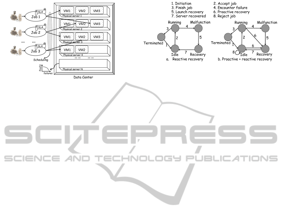
Figure 1: The cloud paradigm.
imization across multiple service level agreements.
Maximizing of the quality of users’ experiences while
minimizing the cost for the provider is studied in
(Mazzucco et al., 2010b). And (Fit´o et al., 2010)
model the economic cost and SLA for moving a web
application to cloud computing. The proposed Cloud
Hosting Provider (CHP) could make use of the out-
sourcing technique for providing scalability and high
availability capabilities, and maximize the providers’
revenue. In contrast to their proposals, our goal is to
improve the cost efficiency of servers by leveraging
the failure prediction methods.
3 SYSTEM MODEL
3.1 Cloud Paradigm
Figure 1 illustrates the basic cloud paradigm. Data
centers consolidate multiple applications to share the
same physical server through virtualization technolo-
gies (Bobroff et al., 2007). VM instances are of-
fered from a diversified catalog with various config-
urations. Jobs are encapsulated into VMs, and cus-
tomers can start new VMs or stop unused ones to
meet the increasing or decreasing workload, respec-
tively, and pay for what they use thereafter. In this
process, customers do not have full control over the
physical infrastructure. Instead, the provider sets a
resource management policy determining the physi-
cal servers for starting VMs. VM instances are com-
monly provided under a single standard availability
SLA: a penalty is punished on the provider if SLA
is violated. During the job execution, a VM may mi-
grate from one physical server to another according to
the policy. We will not discuss the high-level schedul-
ing policy that dispatching VMs to physical servers in
this paper, yet we focus on the low-level management
policy on behalf of a physical server. The proposed
approach could assist high-level scheduling policy in
achieving net revenue improvement.
Figure 2: The state transitions of (a) Reactive recovery and
(b) Proactive-Reactive recovery.
3.2 Job Model
Cloud platform has been employed in a variety of
scenarios, such as scientific computing, web appli-
cation and data storage. The job model abstracted
here mainly comes from the scientific computation.
However, as the presented server management model
solely concerns the contract life between customer
and provider, it is applicable to a diverse spectrum of
application domains. The implementation and evalu-
ations are mainly targeted towards scientific compu-
tational jobs.
Once a job is submitted, the cloud provider dis-
patches the job encapsulated in a VM to a physical
server. The VM’s lifetime could be determined ei-
ther by a user’s specification or job runtime estimates.
In case of user’s specification, we assume the job is
submitted together with the time requirements. In
case of estimate, we use the method of predicting run-
time by searching similar jobs based on the historical
data, e.g., Smith, Foster, and Taylor (1998). Note that
estimating runtime is quite a big challenge, but for-
tunately a moderate-accuracy estimate is acceptable
in our proposal because VM instances are generally
priced by hour. In our evaluations, we choose a rather
simple way to predict runtime, i.e., abstract a job as
a certain amount of workloads, and compute the con-
tract life as the workloads divided by the computa-
tional capacity of a VM.
4 THE POLICY
4.1 Cloud Server Management
A physical server is described with five states as fol-
lows:
IDLE: There are no VMs executing on the server.
RUNNING: The server is executing some VM(s).
TERMINATED: The server successfully finishes
jobs, then recycles the memory and clears the disk.
ONREVENUEDRIVENSERVERMANAGEMENTINCLOUD
297

MALFUNCTION: A failure occurs, and the
server breaks down.
RECOVERY: Troubleshooting, which could be a
simple reboot or repair by a skilled staff.
Figure 2 illustrates the above states and their state
transitions for a physical server. We incorporate
both the MALFUNCTION and RECOVERY into the
states due to the common failures. Although failures
may occur at anytime, the probability of failure oc-
currence in the TERMINATED or IDLE state is far
less than in the RUNNING state. Therefore, a single
in-degree to the MALFUNCTION state is exploited.
Initially, when a new physical server joins a server
farm, or an existing server has finished all deployed
VMs and refreshed his status, the server enters the
IDLE state and becomes ready for serving a next job.
4.1.1 Reactive Recovery
When a job arrives, the server starts a required VM
and accepts the job without hesitation, then comes
into the RUNNING state. In case of a successful ex-
ecution, the job is completed, and the server enters
the TERMINATED state. After clearing the memory
and disk, the server returns to the IDLE state. If a
failure occurs, the server comes into the MALFUNC-
TION state. Certain recovery methods, e.g., repair,
rebooting, would be activated to fix the malfunction,
then the server returns to the IDLE state. Note that
the recovery could be launched by a skilled staff or
automatically activated by a tool like watchdog.
4.1.2 Proactive-reactive Recovery
Proactive recovery is a useful tool for improving the
system efficiency and reducing the economic cost.
However, the effects of proactive recovery heavily de-
pend on the failure prediction accuracy, which is still
in the rough primary stage currently. Therefore, we
employ a hybrid approach based on both proactive re-
covery and reactive recovery here. An architectural
blueprint for managing server system dependability
in a proactive fashion is introduced in Polze, Troger,
and Salfner (2011).
When a job arrives, the server can: 1. accept the
job and change to RUNNING (step 2 in Figure 2(b));
2. reject the job and stay in IDLE (step 8); 3. reject
the job and activate a proactive recovery operation if
a failure is predicted (step 6). To assure a positive net
revenue, we devise a utility function to handle such
decision making problems.
In the first case, if the server comes into the RUN-
NING state, there are three further possible transitions
coming out from the RUNNING state: 1a. if a failure
is anticipated during RUNNING, move all running
Table 1: List of notations.
Notations Definition
Prc
i
Price of the VM instance i ($/hour).
Prc
egy
Price of energy consumption. ($/kw.h)
U
ser
Fixed cost of a physical server ($/hour).
Wgh
i
A weight describing VM i’s percentage of U
ser
.
U
SIO
i
Fixed cost of a VM i. U
SIO
i
= U
ser
·Wgh
i
.
P
i
Energy consumption per time unit for VM i.
Ucoe
i
Task execution cost per time unit. Ucoe
i
= U
SIO
i
+Prc
egy
P
i
T
vm
Job execution time, or contract life.
Coe
i
Total task execution cost of VM i. Coe
i
= Ucoe
i
T
vm
Pen Penalty for SLA violations.
T
M
Time spent on MALFUNCTION state.
T
R
Time spent on RECOVERY state.
P
SLA
The percentage of total bill that the provider has to refund.
P
fail
Probability of failures.
Cmig VM migration cost.
T
rmn
vm
VM’s remaining lifetime.
P
mig
fail
Probability of failures for a migrated VM.
VMs and proactively launch the recovery (step 6);
1b. if a failure occurs without warning, the server re-
actively comes into the MALFUNCTION state (step
4); 1c. if there are no failures, complete the job suc-
cessfully (step 3). A similar utility based function is
also employed here for the proactive recovery opera-
tion. In the second and third cases, the server needs
to decide whether to stay in IDLE state, or activate a
proactive recovery after a job rejection. This is rea-
sonable because a negative net revenue may be ex-
pected from a long-running job, whereas a positive
net revenue is expected from a short-running job. If
the rejected job is a normal or small size one, then the
server activates a proactive recovery, otherwise stays
in the IDLE state.
4.2 Net Revenue
Our net revenue model is similar to those used in the
literature (Mac´ıas et al., 2010; Fit´o et al., 2010) except
that we do not consider the situation of outsourcing a
application to a third-party and hence there is no out-
sourcing cost (Fit´o et al., 2010). Notations are listed
in Table 1.
Price (Prc): is the amount of money that a cus-
tomer has to pay if a cloud provider finishes his job
successfully. It usually takes the time piece as the
unit. For instance, Amazon EC2 standard small in-
stance charges 0.085$ per hour. Cost of execution
(Coe): is the amount of money that a cloud provider
has to spend on maintaining a healthy VM as well as
a physical server for providing service. As the service
providing is the major source of profit, any cost for
maintaining such service providing will be considered
as the part of the total costs, which typically includes
fixed costs (e.g., site infrastructure capital costs, IT
CLOSER2012-2ndInternationalConferenceonCloudComputingandServicesScience
298

capital costs) and variable costs (e.g., energy costs,
operating expenses). Penalty (Pen): is the amount of
money that a provider has to pay if the SLA is vio-
lated. Denote by T
vm
the working time (i.e., contract
life or job execution time), the net revenue obtained
from deploying VM i is computed as below,
Rvu
i
= Prc
i
· T
vm
− Coe
i
− Pen
i
(1)
4.3 Price, Cost and Penalty
The prices of different VM instances have been
clearly announced by the providers, and can be pub-
licly accessed. To calculate the cost of execution,
we must know the total cost of maintaining a cloud
server. Fortunately, the cost model of a data cen-
ter has been studied in (Koomey et al., 2007; Patel
and Shah, 2005; Hoelzle and Barroso, 2009). The
total cost (Toc) of a data center is defined as the
sum of site infrastructure capital costs (Sic), IT capi-
tal costs (Icc), operating expenses (Ope) and energy
costs (Enc): Toc = Sic+ Icc+ Ope+ Enc. In partic-
ular, rates that site infrastructure capital costs take are
most, and IT capital costs (Icc) make up about 33%
of the total cost (P
Icc
= 33%) (Koomey et al., 2007).
We suppose that Sic, Icc and Ope are fixed during the
lifetime of the data center. This is reasonable because
Sic and Icc belong to one time investment, and Ope
does not fluctuate significantly over time. Let lif e
ser
denote the lifetime of a server ser. As the service pro-
viding takes the only source of income of a data cen-
ter, the execution cost of Sic + Icc + Ope amortized
over every server, over lifetime could be roughly esti-
mated as: U
ser
=
Sic+Icc+Ope
N·life
ser
, where N is the number
of servers.
Since multiple VMs are possibly consolidated on
one physical server, U
ser
is supposed to be shared
among VMs, that is, U
SIO
i
= U
ser
· Wgh
i
, where
Wgh
i
= w
cpu
cpu
i
cpu
vms
+ w
ram
ram
i
ram
vms
+ w
disk
disk
i
disk
vms
. w
cpu
,
w
ram
and w
disk
are the weights describing the propor-
tion of CPU, RAM and disk cost, respectively. And
w
cpu
+ w
ram
+ w
disk
= 1. cpu
i
, ram
i
and disk
i
denote
the amount of CPU, RAM, and disk resources allo-
cated to VM i, while cpu
vms
, ram
vms
and disk
vms
rep-
resents the total resources consumed by all VMs de-
ployed on the physical server. Note that Wgh
i
= 1 if
a single VM is deployed on the server.
A server CPU operating at a certain frequency(de-
note by f) consumes dynamic power (P) that is pro-
portional to V
2
· f, where V is the operating voltage
(Chandrakasan, Sheng, and Brodersen, 1995). Since
the operating voltage is proportional to f (i.e., V ∝ f)
and the power consumption of all other components
in the system is essentially constant (denote by a), we
employ the simple model of power consumed by a
VM running at frequency f : P = a+ bf
3
, which has
been used in (Elnozahy et al., 2002) as well. In case of
multiple VMs sharing one server, a is equally divided
among VMs. Therefore, the energy cost for deploy-
ing a VM is Egy = Prc
egy
· P · T
vm
, where Prc
egy
is
the electricity charge per unit of energy consumption.
Denote byUcoe
i
the total execution cost per time unit
for VM i, then Ucoe
i
= U
SIO
i
+ Prc
egy
· P
i
. Therefore,
Coe
i
= Ucoe
i
· T
vm
= (U
SIO
i
+ Prc
egy
· P
i
) · T
vm
(2)
The proposals for measuring the penalty cost
caused by SLA violation vary widely. For exam-
ple, (Fit´o et al., 2010) determine the penalty based
on the time of violation and the magnitude of the vi-
olation. Amazon EC2 compensates customers with
service credit based on the achieved availability level.
In this study, the penalty, caused by SLA violation in
terms of computation jobs, is applied as a refund be-
havior. If the computation job fails due to the server
failures, the cloud provider will not get revenue and
has to pay an extra penalty:
Pen
i
= Prc
i
· T
vm
· P
SLA
(3)
where P
SLA
denotes the fraction of total bill that the
provider has to refund.
4.4 Expected Net Revenue
Now we can compute the expected net revenue from
providing service or possible losses from server fail-
ures. Table 2 shows the probabilities of state tran-
sitions for both the reactive recovery and proactive-
reactive (Figure 2). Table 3 shows all the state transi-
tion paths and the corresponding revenues for both of
them.
In reactive recovery, the cloud server could ob-
tain positive net revenue from job execution in path
1 (denoted as A
R
= (Prc−Ucoe) · T
vm
). While in path
2, the cloud server not only obtains nothing due to
the failure, but also has to pay the penalty and losses
the execution cost. Let T
M
and T
R
be the time spent
on MALFUNCTION and RECOVERY state respec-
tively, then B
R
= U
SIO
(T
vm
+ T
M
+ T
R
) + Prc
egy
· P ·
T
vm
+ Prc· T
vm
· P
SLA
.
In the proactive-reactiverecovery, the cloud server
shows a similar situation in path 1 and path 2, that is
A
PR
= A
R
and B
PR
= B
R
, but with different probabili-
ties. In path 3, a proactive recovery is activated during
the running process. The running VMs are interrupted
and moved to other healthy servers, where they sub-
sequently proceed until finish. During this process,
the cloud provider eventually gets the revenue from
these jobs. The revenue generated in terms of the old
ONREVENUEDRIVENSERVERMANAGEMENTINCLOUD
299

Table 2: The state transition probability for Reactive/Proac-
tive-reactive recovery.
Running Idle Terminated Malfunction Recovery
Running 0/0 0/0 P
′
02
/P
02
P
′
03
/P
03
0/P
04
Idle 1/P
10
0/P
11
0/0 0/0 0/P
14
Terminated 0/0 1/1 0/0 0/0 0/0
Malfunction 0/0 0/0 0/0 0/0 1/1
Recovery 0/0 1/1 0/0 0/0 0/0
Table 3: The server running paths and their corresponding
net revenues.
Reactive recovery Revenue
Path 1 IDLE - RUNNING - TERMINATE - IDLE A
R
Path 2 IDLE - RUNNING - MALFUNCTION - RECOVERY - IDLE −B
R
Proactive-Reactive recovery
Path 1 IDLE - RUNNING - TERMINATE - IDLE A
PR
Path 2 IDLE - RUNNING - MALFUNCTION - RECOVERY - IDLE −B
PR
Path 3 IDLE - RUNNING - RECOVERY - IDLE C
PR
Path 4 IDLE - IDLE 0
Path 5 IDLE - RECOVERY - IDLE −D
PR
server is computed based on the finished fraction of
the total workload, denoted by P
fnd
, therefore, we
have C
PR
= P
fnd
(Prc− Ucoe)T
vm
− U
SIO
T
R
. In path
4 and 5, a job rejection operation only implies a lo-
cal server’s decision, and the rejected job is eventu-
ally accepted by another healthy server from the per-
spective of cloud provider. Thus, there are no losses
caused from the job rejection. And the recovery cost
spent on the proactive recovery operation in path 5 is:
D
PR
= U
SIO
T
R
.
According to Table 2 and Table 3, the expected net
revenue generated by reactive recovery is:
Rvu
R
= A
R
P
′
02
− B
R
P
′
03
(4)
The expected net revenue generated by proactive-
reactive recovery is:
Rvu
PR
= A
PR
P
10
P
02
− B
PR
P
10
P
03
+C
PR
P
10
P
04
− D
PR
P
14
(5)
Theorem 1. Rvu
PR
> Rvu
R
.
Proof.
Rvu
PR
− Rvu
R
= PrcT
vm
×
[P
SLA
(P
′
03
− P
10
P
03
) + (P
10
P
02
− P
′
02
) + P
fnd
P
10
P
04
]+
U
SIO
[T
vm
(P
′
03
− P
10
P
03
− P
fnd
P
10
P
04
+ P
′
02
− P
10
P
02
)+
T
M
(P
′
03
− P
10
P
03
) + T
R
(P
′
03
− P
10
(P
03
+ P
04
) − P
14
)]+
Prc
egy
PT
vm
[P
′
02
− P
10
P
02
+ P
′
03
− P
10
P
03
− P
fnd
P
10
P
04
]
(6)
With the two prerequisites, P
10
P
02
= P
′
02
and P
10
·
(P
03
+ P
04
) + P
11
+ P
14
= P
′
03
, we have,
• P
SLA
(P
′
03
− P
10
P
03
) + (P
10
P
02
− P
′
02
) + P
fnd
P
10
P
04
>
0
•
T
vm
(P
′
03
− P
10
P
03
− P
fnd
P
10
P
04
+ P
′
02
− P
10
P
02
)+
T
M
(P
′
03
− P
10
P
03
) + T
R
(P
′
03
− P
10
(P
03
+ P
04
) − P
14
)
> 0
• P
′
02
− P
10
P
02
+ P
′
03
− P
10
P
03
− P
fnd
P
10
P
04
> 0
Hence, the theorem is established.
4.5 Decision Making
The server state transitions contain three decision
making points. The first one is to decide whether
to accept or reject a new arriving job, and followed
by a further decision is on whether or not to activate
proactive recovery if the job is rejected. The third one
is to decide whether to activate a proactive recovery
or continue the job execution when the job is under
the RUNNING state. In our proposal, these decisions
are made on behalf of physical servers based on the
expected net revenue.
4.5.1 Accept or Reject a Job
A job arriving at a cloud server could be a new or
rejected or failed or migrated job. After its lifetime
(i.e., T
vm
) is determined by user’s specification or es-
timates, we can predict the probability of failures (i.e.,
P
fail
) in this interval using associated stressors (Ajith
and Grosan, 2005). The possible net revenue obtained
from accepting a job by server i can be computed as,
Rvu
i
= A
i
PR
· (1− P
fail
) (7)
Accounting of malfunction losses during the mid-
dle of job execution consists of direct economic loss
and indirect economic loss. A cloud provider would
directly get a penalty from the SLA agreement, and
he also has to afford the cost for recovery operation.
The possible losses can be computed as,
Los
i
= B
i
PR
· P
fail
(8)
If Rvu
i
> Los
i
, the VM i will be deployed for exe-
cution, and if not, the VM i will be rejected. In other
words, the VM i is accepted when the following con-
dition is held,
P
fail
<
A
i
PR
A
i
PR
+ B
i
PR
(9)
In case of a migrated VM, additional cost is spent
on VM migration. Let Cmig be the cost for moving
the VM from an old physical server to a new one, and
T
rmn
vm
be the remaining lifetime. We have,
Rvu
mig
i
= (A
i,rmn
PR
− Cmig) · (1− P
mig
fail
)
= ((Prc
i
− Ucoe
i
) · T
rmn
vm
− Cmig) · (1− P
mig
fail
)
and,
Los
mig
i
= (B
i,rmn
PR
+Cmig) · P
mig
fail
= (Pen
i
+U
SIO
(T
rmn
vm
+ T
M
+ T
R
)+
Prc
egy
· P· T
rmn
vm
+Cmig)P
mig
fail
CLOSER2012-2ndInternationalConferenceonCloudComputingandServicesScience
300

Let Rvu
mig
i
> Los
mig
i
, then the condition 9 is
changed into,
P
mig
fail
<
A
i,rmn
PR
− Cmig
A
i,rmn
PR
+ B
i,rmn
PR
(10)
4.5.2 Proactive Recovery or Not
Once a job is rejected, a cloud server further has two
options of launching the proactive recovery or doing
nothing. Denote by T
vm
the average lifetime of all
history VMs successfully completed on a server, and
P
T
vm
fail
the predicted probability of failures within next
T
vm
time. Then if P
T
vm
fail
< P
fail
(The right side of In-
equality 9), the cloud server does nothing but waits
for the next job. Otherwise, the server activates the
proactive recovery. This is because failure probabil-
ity increases over time. A next normal size job still
can be accepted if P
T
vm
fail
< P
fail
is held. Note that it is
possible that the server stays in a starvation state for a
long time, if no short-running VM is dispatched to the
server. In such case, activate the proactive recovery if
the leisure time exceeds a pre-defined threshold.
4.5.3 Activate VM Migaration or Not
For a long-running VM, it is difficult to have an accu-
rate prediction on the failure probability during that
long time. Moreover, certain types of failures al-
ways come with some pathognomonic harbingers. It
is a difficult to predict such failures without particu-
lar harbingers. Therefore, we also activate the failure
prediction during the running process. And proactive
recovery is launched when inequality 9 (inequality 10
if it is a migrated job) is violated for all the local VMs.
The VM migrates from a server i to a server j
only because j can yield a greater net revenue. The
expected revenue obtained from no migration is the
same as Rvu
i
(Equation 7), except that the failure
probability (P
rmn
fail
) is for the remaining lifetime (i.e.,
T
rmn
vm
): Rvu
rmn
i
= A
i,rmn
PR
· (1− P
rmn
fail
) = (Prc
i
−Ucoe
i
)·
T
rmn
vm
· (1 − P
rmn
fail
). The expect net revenue obtained
from a migration has been described as Rvu
j
mig
. Let
Rvu
mig
j
> Rvu
rmn
i
, we have,
P
mig
fail
<
A
i,rmn
PR
· P
rmn
fail
− Cmig
A
i,rmn
PR
− Cmig
(11)
Therefore, a new server j whose failure probabil-
ity (i.e., P
Mig
fail
) follows both Inequality 10 and 11 will
be selected to execute the migrated VM. In case of
more than one server meets this condition, the VM
migrates to the one with maximum reliability to pro-
ceed. If no appropriate processors are found, maintain
the VM at the original server until finish or failure.
5 EXPERIMENTS
5.1 Simulation Environment
5.1.1 Server Farm
We simulate a server farm with 20 physical servers,
which can provide seven different types of VM in-
stances, corresponding to the seven types of instances
from Rackspace Cloud Servers (Rackspace, 2012).
The processing speed of each server is supposed to
be the same, and is initialized with eight cores, with
each is of 2.4GHz.
5.1.2 Job
We simulate a large number of jobs ranging from
1000 to 6000, for maximizing the utilization of all
servers. Through this way, the cost for maintaining
a server could be fairly shared among all the VMs
deployed on it, and leading to a positive net rev-
enue. This is also reasonable in practice because
cloud providers commonly design policies to opti-
mize the minimum number of active servers for re-
ducing the energy cost, thereby resulting in a high uti-
lization at each active server (Mastroianni, Meo, and
Papuzzo, 2011; Mazzucco et al., 2010b).
Allowing two instructions in one cycle, the work-
load of each job is evenly generated from the range:
[1, 6] × 204, 800 × 2
i
million instructions, where 0 ≤
i ≤ 6 and i ∈ Z, represents the type of VM instance
this job requires.
5.1.3 Scheduling
Jobs are placed on cloud servers using a First-Come-
First-Served (FCFS) algorithm. Scheduling priority
is supported, and follows the sequence: migrated job
> failed job > rejected job > unsubmitted job. The
rejected or failed jobs will not be scheduled on the
same server at the second time, because it is probably
rejected or failed again.
5.1.4 Failures
Failures are considered from two dimensions. The
first dimension concerns the time when failures oc-
cur. In our experiments, failures are injected to
servers following a Poisson distribution process with
ONREVENUEDRIVENSERVERMANAGEMENTINCLOUD
301

λ = [1, 4]
θ × 10
−6
, where θ ∈ [0.1, 2]. According
to the Poisson distribution, the lengths of the inter-
arrival times between failures follow the exponential
distribution, which is inconsistent with the observa-
tions that the time between failures is well modeled
by a Weibull or lognormal distribution (Schroeder and
Gibson, 2006). The deviations arise because an at-
tempt to repair a computer is not always successful
and failures recur a relatively short time later (Lewis,
1964). Implementing a real failure predictor is out of
the range of this paper, and we alternatively consider
different failure prediction accuracy in evaluations.
The second dimension concerns the repair times.
If an unexpected failure occurs, the server turns into a
MALFUNCTION state immediately, and followed by
recovery operations. As discussed in (Schroeder and
Gibson, 2006), the time spent on recovery follows a
Lognormal distribution process, which is defined with
a mean value equaling to 90 minutes, and σ = 1.
5.1.5 Price and Server Cost
The prices for all seven types of VM instances are set
exactly the same as the ones from Rackspace Cloud
Servers (Rackspace, 2012), that is Prc = 0.015$× 2
i
,
where 0 ≤ i ≤ 6 and i ∈ Z.
The capital cost is roughly set at 8000$ per phys-
ical server, which is estimated based on the market
price of System x 71451RU server by IBM (IBM,
2012). The price of electricity is set at 0.06$ per kilo-
watt hour. We suppose that the power consumption
of an active server without any running VMs is 140
Watts. Additional power ranging from 10 Watts to 70
Watts is consumed by VMs corresponding to seven
types of VM instances (Mazzucco et al., 2010b). Sup-
pose a server’s lifetime is five years, and as the IT cap-
ital cost takes up 33% to the total management cost,
we roughly spend 4300$ on a physical server per year
with additional energy cost.
As modeling of migration costs is highly non-
trivial due to second order effects migrations might
have on the migrated service and other running ser-
vices, we simplify migration costs as an additional
20% of the unexecuted workload without profit (i.e.,
10% for the original server, and another 10% for the
target server). A preliminary attempt on modeling mi-
gration cost is given in Breitgand, Kutiel, and Raz
(2010).
5.1.6 Penalty
If a SLA is breached due to the provider’s failing to
complete jobs, the customer gets compensation by a
rather high ratio of fine, which ranges from 10% to
500% of the user bill in the experiments (i.e., P
SLA
∈
[0.1, 5]). This is because SLA violations cause not
only direct losses on revenue but also indirect losses,
which might be much more significant (e.g., in terms
of provider reputation).
5.2 Results
We choose the evaluation approach by comparing our
proposed proactive-reactive model with the original
reactive model. Experiments are conducted across a
range of operating conditions: number of jobs, fail-
ure frequency (θ), P
SLA
, and the accuracy of failure
prediction. Accuracy implies the ability of the fail-
ure prediction methods, and is presented by both the
false-negative (fn) and false positive (fp) ratio. De-
note by No(FN) the number of false-negative errors,
No(TP) the number of true-positive predictions, and
No(FP) the number of false-positive errors, then we
have fn =
No(FN)
No(FN)+No(TP)
and f p =
No(FP)
No(FP)+No(TP)
.
Unless otherwise stated, the parameters are set with
jobnumber = 1000, θ = 1, P
SLA
= 0.1, fn = 0.25 and
f p = 0.2. Each experiment is repeated five times and
the results represent the corresponding average val-
ues.
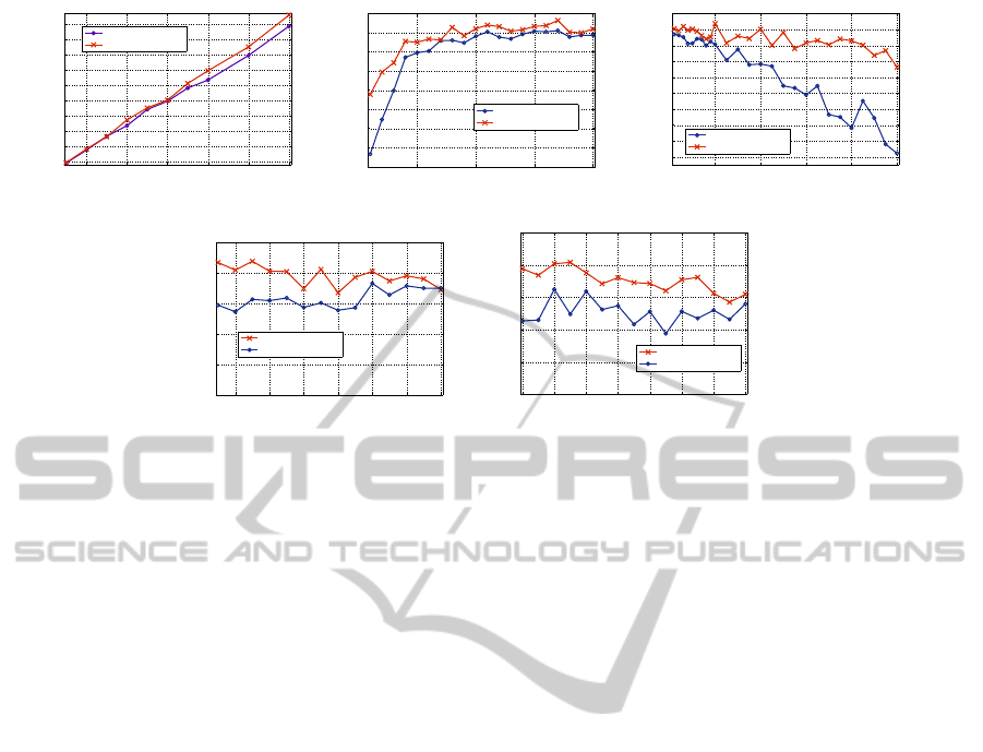
Figure 3 shows the total net revenue obtained by
both the proactive-reactive recovery and reactive re-
covery from executing jobs under different operat-
ing conditions. Generally, net revenue yielded by the
proactive-reactive model is greater than the reactive
model, which is consistent with our analysis in The-
orem 1. In particular, Figure 3(a) shows the net rev-
enue as a function of the number of jobs. The dif-
ference on net revenue is increasing over the number
of jobs, which is reasonable because more jobs come
with more revenue.
Figure 3(b) shows the net revenue as a function
of failure frequency. By the definition of λ, we know
failure frequency decreases as θ increases. As shown
in the figure, the proactive-reactive model could yield
more net revenue than the reactive model when the
failure frequency is high. In particular, the proactive-
reactive model yields 26.8% net revenue improve-
ment over the reactive model when setting θ = 0.1.
And an average improvement of 11.5% is achieved
when θ ≤ 0.5. This suggests that the proactive-
reactive model makes more sense in unreliable sys-
tems. Furthermore, the proactive-reactive model also
outperforms the reactive model in rather reliable sys-
tems where θ > 0.5.
Figure 3(c) shows that the proactive-reactive
model yields a greater net revenue than the reac-
tive model under different P
SLA
values. Net revenue
yielded by the proactive-reactive model does not de-
cline much because most penalty costs are avoided
CLOSER2012-2ndInternationalConferenceonCloudComputingandServicesScience
302
1000 2000 3000 4000 5000 6000
1
2
3
4
5
6
7
8
9
10
x 10
4
Total number of job requests
Total Net Revenue ($)
Reactive
Proactive+Reactive
(a)
0.5 1 1.5 2
1.1
1.2
1.3
1.4
1.5
1.6
1.7
1.8
1.9
x 10
4
Theta (Poisson distribution)
Total Net Revenue ($)
Reactive
Proactive+Reactive
(b)
1 2 3 4 5
0.2
0.4
0.6
0.8
1
1.2
1.4
1.6
1.8
2
x 10
4
P
SLA
Total Net Revenue ($)
Reactive
Proactive+Reactive
(c)
0.1 0.2 0.3 0.4 0.5 0.6 0.7
1.6
1.65
1.7
1.75
1.8
1.85
x 10
4
False negative ratio
Total Net Revenue ($)
Proactive+Reactive
Reactive
(d)
0.1 0.2 0.3 0.4 0.5 0.6 0.7 0.8
1.6
1.65
1.7
1.75
1.8
1.85
x 10
4
False positive ratio
Total Net Revenue ($)
Proactive+Reactive
Reactive
(e)
Figure 3: The total net revenue: (a) under different No. of jobs; (b) under different θs (failure frequency); (c) under different
SLA penalty percentages; (d) under different levels of false-negative ratio; (e) under different levels of false-positive ratio;
by possible proactive recovery and VM migrations.
Whereas the reactive model has to pay the penalty
when failure occurs, and penalty cost increases as
P
SLA
increases.
Figure 3(d) shows the net revenue under different
levels of false-negative ratio ranging from 0.05 to 0.7.
With the increase of false-negative error, there is a
slight decrease on the net revenue by the proactive-
reactive model, whereas the reactive model fluctu-
ates around a certain level because the reactive model
does not employ failure prediction and the fluctua-
tion is due to the random values used in the experi-
ments. Our proactive-reactivemodel averagely yields
3.2% improvement on the net revenue over the re-
active model, and performs similarly with reactive
model when fn ≥ 0.7.
Figure 3(e) shows the impact on net revenue from
the false-positive ratio under a fixed fn = 0.25. Net
revenue obtained from proactive-reactive model de-
creases gradually over the false positive ratio. More-
over, the differences on revenue between proactive-
reactive and reactive model decreases as the false-
positive ratio increases. This is because a high false-
positive ratio results in a large number of meaningless
migrations, which come with migration costs. Figure
3(d) and Figure 3(e) suggest that our algorithm still
performs well with even modest prediction accuracy
(i.e., fn ≥ 0.5 or f p ≥ 0.5).
6 CONCLUSIONS
A major reason for the rapid development of cloud
computingrests with its low cost to deploy customers’
applications. As long as customers pay a small fee to
providers, they can access and deploy their applica-
tions on the cloud servers. Cloud computing frees
them from the complicated system installment and
management, and even allows them to expand or con-
tract their requirements smoothly. In this context, op-
timizing cloud systems from an economics perspec-
tive will further reduce costs of services, and hence
improve the cost efficiency of cloud.
In this paper, we address the problem of cost-
efficient fault management, and present a revenue
driven server management model for cloud systems.
Using this model, cloud providers could obtain a sig-
nificant improvementon net revenuewhen serving the
same jobs. In particular, our proposal could yield at
most 26.8%, on average 11.5% net revenue improve-
ment when the failure frequency is high. Moreover,
because our proposal works on the rock-bottom level
and do not modify the existing upper cloud systems, it
can be easily incorporated into current cloud systems.
In the future, we will study the performances
of different scheduling algorithms working together
with the proposed server management model. Our
goal is to maximize the net revenue for cloud
providers without affecting the performance.
ACKNOWLEDGEMENTS
The first author of this research is supported by
the governmentalscholarship from China Scholarship
Council. We would like to thank the anonymous re-
ONREVENUEDRIVENSERVERMANAGEMENTINCLOUD
303

viewers for their valuable suggestions on how to im-
prove the quality of this paper.
REFERENCES
Ajith, A. and Grosan, C. (2005). Genetic programming ap-
proach for fault modeling of electronic hardware. In
The 2005 IEEE Congress on Evolutionary Computa-
tion, CEC’05, pages 1563–1569. IEEE.
AmazonSLA (2012). Amazon ec2 service level agreement.
Retrieved Jan. 31, 2012, from http://aws.amazon.com/
ec2-sla/.
AzureSLA (2012). Microsoft azure compute service level
agreement. Retrieved Jan. 31, 2012, from http://
www.windowsazure.com/en-us/support/sla/.
Bobroff, N., Kochut, A., and Beaty, K. (2007). Dynamic
Placement of Virtual Machines for Managing SLA Vi-
olations. 10th IFIP/IEEE International Symposium on
Integrated Network Management, pages 119–128.
Breitgand, D., Kutiel, G., and Raz, D. (2010). Cost-aware
live migration of services in the cloud. In Proceedings
of the 3rd Annual Haifa Experimental Systems Con-
ference, SYSTOR ’10, pages 11:1–11:6, New York,
USA. ACM.
Chandrakasan, A. P., Sheng, S., and Brodersen, R. W.
(1995). Low power cmos digital design. IEEE Journal
of Solid State Circuits, 27:473–484.
Dean, J. (2006). Experiences with mapreduce, an abstrac-
tion for large-scale computation. In Proceedings of
the 15th international conference on Parallel archi-
tectures and compilation techniques, PACT ’06, pages
1–1, New York, NY, USA. ACM.
Elnozahy, E. M., Kistler, M., and Rajamony, R. (2002).
Energy-efficient server clusters. In Proceedings of the
2nd Workshop on Power-Aware Computing Systems,
pages 179–196.
Fit´o, J. O., Presa, I. G., and Guitart, J. (2010). Sla-
driven elastic cloud hosting provider. In Proceedings
of the 2010 18th Euromicro Conference on Parallel,
Distributed and Network-based Processing, PDP ’10,
pages 111–118, Washington, DC, USA. IEEE Com-
puter Society.
Fu, S. and Xu, C. Z. (2007). Exploring event correlation for
failure prediction in coalitions of clusters. In Proceed-
ings of the 2007 ACM/IEEE conference on Supercom-
puting, SC ’07, pages 41:1–41:12, New York, USA.
ACM.
GoogleSLA (2012). Google apps ec2 service level
agreement. Retrieved Jan. 31, 2012, from http://
www.google.com/apps/intl/en/terms/sla.html.
Hoelzle, U. and Barroso, L. A. (2009). The Datacenter
as a Computer: An Introduction to the Design of
Warehouse-Scale Machines. Morgan and Claypool
Publishers, 1st edition.
IBM (2012). Ibm system x 71451ru entry-level server. Re-
trieved Jan. 31, 2012, from http://www.amazon.com/
System- 71451RU- Entry- level- Server- E7520/dp/
B003U772W4.
Koomey, J., Brill, K., Turner, P., Stanley, J., and Taylor, B.
(2007). A simple model for determining true total cost
of ownership for data centers. Uptime institute white
paper.
Lewis, P. A. (1964). A branching poisson process model
for the analysis of computer failure patterns. Journal
of the Royal Statistical Society, Series B, 26(3):398–
456.
Mac´ıas, M., Rana, O., Smith, G., Guitart, J., and Torres,
J. (2010). Maximizing revenue in grid markets using
an economically enhanced resource manager. Con-
currency and Computation Practice and Experience,
22:1990–2011.
Mao, M., Li, J., and Humphrey, M. (2010). Cloud auto-
scaling with deadline and budget constraints. In 11th
IEEE/ACM International Conference on Grid Com-
puting, pages 41–48. IEEE.
Mastroianni, C., Meo, M., and Papuzzo, G. (2011). Self-
economy in cloud data centers: statistical assignment
and migration of virtual machines. In Proceedings
of the 17th international conference on Parallel pro-
cessing - Volume Part I, Euro-Par’11, pages 407–418,
Berlin, Heidelberg. Springer-Verlag.
Mazzucco, M., Dyachuk, D., and Deters, R. (2010a). Maxi-
mizing cloud providers’ revenues via energy aware al-
location policies. In Proceedings of the 2010 IEEE
3rd International Conference on Cloud Computing,
CLOUD ’10, pages 131–138, Washington, DC, USA.
IEEE Computer Society.
Mazzucco, M., Dyachuk, D., and Dikaiakos, M. (2010b).
Profit-aware server allocation for green internet ser-
vices. In Proceedings of the 2010 IEEE Interna-
tional Symposium on Modeling, Analysis and Simu-
lation of Computer and Telecommunication Systems,
MASCOTS ’10, pages 277–284, Washington, DC,
USA. IEEE Computer Society.
Nightingale, E. B., Douceur, J. R., and Orgovan, V. (2011).
Cycles, cells and platters: an empirical analysisof
hardware failures on a million consumer pcs. In Pro-
ceedings of the sixth conference on Computer systems,
EuroSys ’11, pages 343–356, New York, NY, USA.
ACM.
Patel, C. D. and Shah, A. J. (2005). A simple model for
determining true total cost of ownership for data cen-
ters. Hewlett-Packard Development Company report
HPL-2005-107, pages 1–36.
Pinheiro, E., Weber, W. D., and Barroso, L. A. (2007). Fail-
ure trends in a large disk drive population. In Proceed-
ings of the 5th USENIX conference on File and Stor-
age Technologies, pages 17–28, Berkeley, CA, USA.
USENIX Association.
Polze, A., Troger, P., and Salfner, F. (2011). Timely
virtual machine migration for pro-active fault toler-
ance. In Proceedings of the 2011 14th IEEE Inter-
national Symposium on Object/Component/Service-
Oriented Real-Time Distributed Computing Work-
shops, ISORCW ’11, pages 234–243, Washington,
DC, USA. IEEE Computer Society.
Rackspace (2012). Rackspace cloud servers. Retrieved Jan.
31, 2012, from http://www.rackspace.com.
Salfner, F., Lenk, M., and Malek, M. (2010). A survey
CLOSER2012-2ndInternationalConferenceonCloudComputingandServicesScience
304

of online failure prediction methods. ACM Comput.
Surv., 42:10:1–10:42.
Schroeder, B. and Gibson, G. A. (2006). A large-scale
study of failures in high-performance computing sys-
tems. In Proceedings of the International Conference
on Dependable Systems and Networks, pages 249–
258, Washington, DC, USA. IEEE Computer Society.
Smith, W., Foster, I. T., and Taylor, V. E. (1998). Pre-
dicting application run times using historical informa-
tion. In Proceedings of the Workshop on Job Schedul-
ing Strategies for Parallel Processing, pages 122–142,
London, UK. Springer-Verlag.
Vishwanath, K. V. and Nagappan, N. (2010). Characteriz-
ing cloud computing hardware reliability. In Proceed-
ings of the 1st ACM symposium on Cloud computing,
SoCC ’10, pages 193–204, New York, USA. ACM.
ONREVENUEDRIVENSERVERMANAGEMENTINCLOUD
305
