EXPLORING mEMD FOR FACE RECOGNITION
Esteve Gallego-Jutglà and Jordi Solé-Casals
Digital Technologies Group, University of Vic, Sagrada Família 7, 08500 Vic, Spain
Keywords: Face Recognition, Multivariate Empirical Mode Decomposition (mEMD), Biometrics.
Abstract: Face recognition is a common technique used for security environment. In this work we explore the
multivariate empirical mode decomposition as technique for face recognition tasks. An image classification
method based on this decomposition is presented and tested. Images are decomposed and then classified
based on the distance between the image and the representative image of each class. Three different
possibilities are presented for compute the distance measures. Preliminary results (82,50 % of classification
rate) are satisfactory and will justify a deep investigation on how to apply mEMD for face recognition.
1 INTRODUCTION
Nowadays, several security laws have been
proposed. As a result, the control of the environment
has increased in different places, such as airports,
train stations and underground stations, border
crossings between countries, governmental
buildings, etc. To control these environments,
different biometric systems are being used.
One of those systems is face recognition. This
system has become one of the biggest challenges in
technological development, due to the relevance that
these applications have achieved. Different fields
have benefited from the use of face recognition, such
as continuous monitoring, access security,
telecommunication systems, etc. (Woodward et al.,
2003, Xiao, 2007).
Face recognition has been quickly developed,
and it seems that there is not a limit for the capacity
of this system, because the data entry of these
systems can be really big. This is why researchers
try to improve the existent systems introducing new
characteristics and new working lines that can be
valid for the developing of these kinds of systems
(Iancu et al., 2007).
Face recognition is a non invasive method. This
supposes an advantage compared with other
systems, which require the guide collaboration of the
subjects that form the data base. The data capture is
also easier with this method.
This paper explores a promising strategy for face
recognition, using a new decomposition technique,
the multivariate empirical mode decomposition.
Images of the subjects are decomposed and
compared before the classification is performed.
This paper is organized as follows: After this
introduction, the used database is presented in
section 2. EMD technique is presented in Section 3,
and its extension for multivariate signals is presented
in Section 4. Section 5 is devoted to the proposed
image processing methodology. Experiments and
results are shown in Section 6 and discussed in
section 7. Finally, conclusions are presented in
Section 8.
2 DATABASE
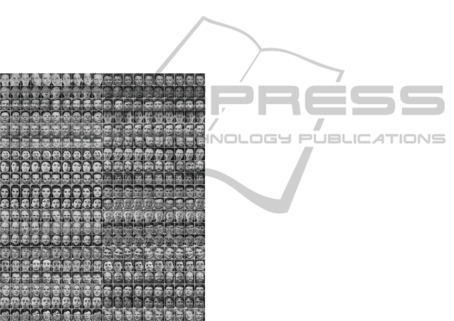
The used database contains ten different images of
forty subjects, which represents a total of four
hundred different images. Images were taken with a
dark background, in a frontal position but with
different orientations of the head in all of them. The
whole dataset is presented in Figure 1.
This database presents images with different
gestural positions, such as eyes open eyes close,
smile non-smile, glasses non-glasses and
illumination variations. The illumination variations
are not defined. All images are grey scale of 256
values, with a size of 92 x 112 pixels.
3 EMPIRICAL MODE
DECOMPOSITION (EMD)
EMD algorithm is a method designed for multiscale
498
Gallego-Jutglà E. and Solé-Casals J..
EXPLORING mEMD FOR FACE RECOGNITION.
DOI: 10.5220/0003894004980503
In Proceedings of the International Conference on Bio-inspired Systems and Signal Processing (MPBS-2012), pages 498-503
ISBN: 978-989-8425-89-8
Copyright
c
 2012 SCITEPRESS (Science and Technology Publications, Lda.)

decomposition and time –frequency analysis, which
can analyze nonlinear and non-stationary data
(Huang et al., 1998).
The key part of the method is the decomposition
part in which any time-series data set can be
decomposed into a finite and often small number of
Intrinsic Mode Functions (IMFs). These IMFs are
defined so as to exhibit locality in time and to
represent a single oscillatory mode. Each IMF
satisfies two basic conditions: (i) the number of
zero-crossings and the number of extrema must be
the same or differ at most by one in the whole
dataset, and (ii) at any point, the mean value of the
envelope defined by the local maxima and the
envelope defined by the local minima is zero (Huang
et al., 1998).
Figure 1: Data base ORL (Olivetti Research Laboratory).
The EMD algorithm (Huang et al., 1998) for the
signal 
(

)
can be summarized as follows.
(i) Determine the local maxima and minima
of

(

)
;
(ii) Generate the upper and lower signal
envelope by connecting those local maxima and
minima respectively by an interpolation method;
(iii) Determine the local mean


(

)
, by
averaging the upper and lower signal envelope;
(iv) Subtract the local mean from the data:
ℎ

(

)
=
(

)
−

(

)
.
(v) If ℎ

(

)
 obeys the stopping criteria, then
we define
(

)
=ℎ

(

)
as an IMF, otherwise set

(

)
=ℎ

(

)
and repeat the process from step (i).
Then, the empirical mode decomposition of a
signal
(

)
can be written as:
x
(
t
)
=IMF

(
t
)
+ε

(
t
)


(1)
Where n is the number of extracted IMFs, and the
final residue ε

(
t
)
is the mean trend or a constant.
4 MULTIVARIATE EMPIRICAL
MODE DECOMPOSITION
(MEMD)
EMD has achieved optimal results in data processing
(Diez et al., 2009, Molla et al., 2010). However, this
method presents several shortcomings in
multichannel datasets. The IMFs from different time
series do not necessarily correspond to the same
frequency, and different time series may end up
having a different number of IMFs. For
computational purpose, it is difficult to match the
different obtained IMFs from different channels
(Mutlu and Aviyente, 2011).
To solve these shortcomings, an extension of
EMD to mEMD is required. In this approach the
local mean is computed by tanking an average of
upper and lower envelopes, which in turn are
obtained by interpolating between the local maxima
and minima. However, in general, for multivariate
signals, the local maxima and minima may not be
defined directly. To deal with these problems
multiple n-dimensional envelopes are generated by
taking signal projections along different direction in
n-dimensional spaces (Rehman and Mandic, 2010).
mEMD is the technique used in this paper to
compute all the decompositions.
The algorithm (Rehman and Mandic, 2010) can
be summarized as follows.
(i) Choose a suitable point set for sampling
on an
(
−1
)

sphere (this
(
−1
)

sphere resides in an
 dimensional Euclidean coordinate system).
(ii) Calculate the projection,
p


(
t
)



, of the
input signal v
(
t
)


along the direction vector,
x


for all k giving p


(
t
)



.
(iii) Find the time instants t



corresponding to
the maxima of the set of projected signals
p
θ
k
(
t
)
t=1
T
.
(iv) Interpolate
t



,vt



 to obtain multivariate
envelope curves
e


(
t
)



.
(v) For a set of K direction vectors, the mean
of the envelope curves is calculated as

(
t
)
=
(
1K
⁄)∑
e


(
t
)


EXPLORING mEMD FOR FACE RECOGNITION
499

(vi) Extract the detail

(

)
using

(

)
=
(

)
−
(

)
. If the detail 
(

)
fulfills the
stopping criteria for a multivariate IMF, apply the
above procedure to
(

)
−
(

)
, otherwise apply it
to 
(

)
.
Then, the mEMD of a signal x
(

)
can be written
as detailed in equation 1.
5 IMAGE PROCESSING
The proposed procedure is detailed in Figure 2. The
system works as follow:
(i) The first 5 images are kept as
representative for each class and the mean image of
these 5 images is obtained for each class. These
images will be named as R

∀1 ≤ i ≤ N, where N is
the total number of classes.
(ii) The rest of the images will be used to be
classified as belonging to one of the forty classes.
(iii) For each new input image I to be
classified, mEMD decomposition between I and R

is calculated, obtaining a total of N mEMD
decompositions:
D

= mEMD(R

, I) ∀1 ≤  ≤ 
(2)
Each one of these D

decompositions is composed by
two sets (matrix) of IMFs, one set (matrix)
belonging to I and the other belonging to R

, and
each IMF have 340 points, where 340 is derived as
20*17 (unfolding an image to a vector, taking into
account that the original size of each image has been
reshaped to 20 x 17).
(iv) Then the distance between IMFs is
calculated for each D
i
, obtaining a vector of N
values corresponding to the distances between input
image I and each one of the classes.
(v) The input image I is associated to the class
corresponding to the minimum distance.
Concerning distance measures, we have explored
different possibilities. Considering two matrix A and
B, corresponding to the obtained two sets of IMFs,
(D
i
) we can propose to use the following measures:
(i) Correlation coefficient between matrices A
and B. That is, the linear correlation coefficient
between A(:) and B(:) (where (:) stands for
unfolding the matrix to a vector)
(ii) Matrix scalar product, also known as the
normalized Frobenius inner product:

(

,
)
=

:
‖

‖

‖

‖

(3)
Figure 2: Scheme of the proposed image processing
procedure.
Where A:B is the the Frobenius inner product of the
matrices A and B, defined as A:B = trace(A

B),
and
‖
·
‖

is the Frobenius norm defined as
‖
A
‖

=


trace(A

A), where
T
denotes the transpose of a
matrix.
(iii) Frobenius norm of the differenceA−B:

(

,
)
=
‖

−
‖

(4)
6 EXPERIMENTS
Initially, as explained before, each image is resized
to 20 x 17. With that we try to find a good
relationship between computational time and
performance.
Applying the detailed procedure to the images,
and using the described three different distances
measures, we obtain the following results:
a) Correlation distance: 41 faces where
misclassified, obtaining therefore a
classification rate of 79,50 %. Confusion
matrix is shown in Figure 3.
b) Matrix scalar product: 39 faces where
misclassified, obtaining therefore a
classification rate of 80,50 %. Confusion
matrix is shown in Figure 4.
c) Frobenius norm: product: 35 faces where
misclassified, obtaining therefore a
classification rate of 82,50 %. Confusion
matrix is shown in Figure 5.
BIOSIGNALS 2012 - International Conference on Bio-inspired Systems and Signal Processing
500

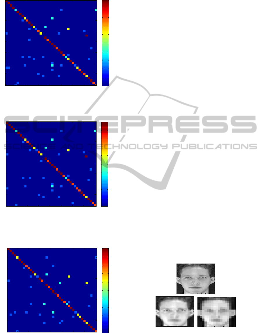
Figure 3: Confusion matrix for the correlation distance
measure. Dark colour indicates good classification (5 over
5 images well classified) for the given class.
Figure 4: Confusion matrix for the matrix scalar product
distance measure. Dark colour indicates good
classification (5 over 5 images well classified) for the
given class.
Figure 5: Confusion matrix for the Frobenius norm
distance measure. Dark colour indicates good
classification (5 over 5 images well classified) for the
given class.
As can be seen, the best result is obtained with
the 3th proposed distance measure, the Frobenius
norm distance.
Comparing this result with results obtained in
(Travieso et al., 2007) we can see that we are clearly
below (82,50 % again 98%), but in (Travieso et al.,
2007) a DCT or DWT (Biorthonal 4.4 family)
parameterization was used combined with an SVM
classifier.
After this first experiment, we focus our
attention in some specific IMFs of the images, trying
to discover if some of them can be removed before
computing the distance between images. Following
this idea, we repeat the previous experiment but
taking into account only some of the IMFs and the
Frobenius norm as a distance measure. We start
eliminating low frequency modes in all the mEMD
decompositions, and the best result is obtained using
the four first modes of each image, which who we
obtain similar performance: 82%. In this sense we
can conclude that the most important information
needed for image classification is located in the
medium and high frequencies.
If we look in detail where the errors are located,
we realize that they are specially produced by
subject 14 (4 errors over 5 images), subject 17 (5
errors over 5 images) and subject 31 (4 errors over 5
images). The same subjects are misclassified using
only the first 4 IMFs. Interestingly, all those 3
subjects wear glasses but not in all the images.
Our last experiment focuses in the repetition of
the first experiment but using larger images. In this
case, we resize the original images to 29 x 34 pixels.
The choice of this size is justified in order to have
the same number of parameters (986 pixels) as in in
(Travieso et al., 2007), giving us the possibility to
compare performances. This larger size keeps much
more information of the image, as it can be seen in
Figure 6.
Figure 6: Example of an original image (top), and the
same resized image (down). Down-left image has 29 x 34
pixels, whereas down-right image has 17 x 20 pixels.
Applying our proposed system to the first 10
5 10 15 20 25 30 35 40
5
10
15
20
25
30
35
40
0
0.5
1
1.5
2
2.5
3
3.5
4
4.5
5
5 10 15 20 25 30 35 40
5
10
15
20
25
30
35
40
0
0.5
1
1.5
2
2.5
3
3.5
4
4.5
5
5 10 15 20 25 30 35 40
5
10
15
20
25
30
35
40
0
0.5
1
1.5
2
2.5
3
3.5
4
4.5
5
10 20 30 40 50 60 70 80 90
10
20
30
40
50
60
70
80
90
100
110
5 10 15 20 25 30
5
10
15
20
25
2 4 6 8 10 12 14 16
2
4
6
8
10
12
14
16
18
20
EXPLORING mEMD FOR FACE RECOGNITION
501

subjects, and using the Frobenius norm as a distance
measure, obtained results rise up to 98% of
classification rate, at the same level of (Travieso et
al., 2007). Confusion matrix is presented in Figure 7.
Figure 7: Confusion matrix for the Frobenius norm
distance measure, image size of 17 x 20 pixels and only
the first 10 subjects of the database. Dark colour indicates
good classification (5 over 5 images well classified) for
the given class. Only one image was misclassified.
Using larger images, the system becomes slower,
and this is a point to take into account. Processing
one image takes some minutes (typically about 4 or
5 min), as the mEMD decomposition is hard to
compute for large vectors. This is one drawback at
this moment, but it can be overcome improving the
mEMD routine or using faster processing hardware.
7 DISCUSSION
Performance results obtained with images at 17 x 20
pixels are quite good if we take into account that the
original images have 10.304 pixels (92 x 112) and
now we have only 340 pixels (applied factor
reduction is about 30).
The experiment performed with larger images
confirms that the system could be interesting in
order to select features of the images. In this case,
for the first 10 subjects, we fail only in one case.
Using the first 10 subjects of the first experiment
(images of 17 x 20 pixels) as a reference, we
decrease the number of errors from 4 to 1, thus we
could expect a similar proportion for the rest of the
images. In this case, the final performance would be
of 95,5%, that is similar to that obtained with other
systems.
Concerning calculation speed, and at this
moment, this system is not suitable for real time
implementations, due to the computational load of
the mEMD decomposition that dramatically
increases with the number of points. This is why we
try to maintain a very low number of pixels of the
images.
Taking into account the previous remark about
computational load, another interesting thing to
discuss is the classification system used. In this work
we focus only in a simple distance measure between
IMFs. Of course, the use of powerful classification
systems like Neural Networks of SVM can be
investigated, as they can help to obtain better results,
but it was out of the scope of this preliminary work.
At this point, images size of 17 x 20 can maybe be
used, combined with an SVM classification system
in order to improve the performance. We will
investigate these and other possibilities in future
works.
8 CONCLUSIONS
The explored method for face classification
presented in this work is based on mEMD technique,
and uses only distance measures to decide to which
class one input image belongs.
Using mEMD, two different matrices are
obtained, containing the different IMF’s, one of
them belonging to the input image to be classified
and the other one to one of the classes. Calculating
the distance between these two matrices, and thus
having a vector of distances from the input image to
all the classes, we associate the class to whom the
input image belongs to that is close to this image, i.e.
to which one that has minimum distance.
We try thee different distance measures
(correlation, matrix scalar product and Frobenius
norm), and the Frobenius norm distance measure
gave the best results. On the other hand, we try also
different image resolutions in order to see if we can
work with very low resolution images that will
increase calculation speed, a necessary condition for
real time application. Working with images of 17 x
20 pixels we obtained 82,5% of classification rate.
Using larger images (29 x 34 pixels) and the first 10
subjects of the database, the performance increases
up to 98%, results comparable to that obtained by
other authors.
The success of the proposed method is promising
and will encourage us to continuing investigating the
use of mEMD decomposition as a feature extracting
system for face recognition problems, combined
with powerfull classification systems like Neural
Networks or SVM.
2 4 6 8 10
1
2
3
4
5
6
7
8
9
10
0
0.5
1
1.5
2
2.5
3
3.5
4
4.5
5
BIOSIGNALS 2012 - International Conference on Bio-inspired Systems and Signal Processing
502

ACKNOWLEDGEMENTS
This work has been partially supported by the
University of Vic under the grant R0904.
REFERENCES
Travieso, C. M., Solé-Casals, J., Zaiats, V., Alonso, J. B.,
Ferrer, M. A., “Reducción del Vector de
Características en Reconocimiento Facial”, XXIII
Simposium Nacional de la Unión Científica
Internacional de Radio URSI 2008.
Diez, P. F., Mut, V., Laciar, E., Torres, A., Avilla, E.
(2009). Application of the Empirical Mode
Decomposition to the Extraction of Features form
EEG signals for Mental Task Classification. 31
st
Annual International Conference of the IEEE EMBS.
Huang, N. E., Shen, Z., Long, S. R., Wu, M. C., Shih, H.
H:, Zheng, Q., Yen, N. C., Tung, C. C., Liu, H. H.
(1998). The empirical mode decomposition and the
Hilbert spectrum for nonlinear and non-stationary time
series analysis. Proc. R. Soc. Lond., 495, 2317-2345.
Iancu, C., Corcoran, P., Costache, G. (2007). A Review of
Face Recognition Techniques for In-Camera
Applications. International Symposium on Signals,
Circuits and Systems, 1, 1-4.
Molla, K. I., Tanaka, T., Rutkowski, T. M., Cichocki, A.,
(2010). Separation of EOG artifacts from EEG singals
using bivariate EMD. Acoustics Speech and Signal
Processing (ICASSP), 2010 IEEE Interational
Conference On. 562-565.
Mutlu, A. Y., Aviyente, S. (2011). Mutivariate Empirical
Mode Decomposition for Quantifying Multivariate
Phase Synchronization. EURASIP Jounal on Advances
in Signal Processing. Article ID 615717
Rehman, N., Mandic, D. P., (2010). Multivariate empirical
mode decomposition. Proc. R. Soc. A. 466, 1291-
1302.
Woodward, J. D., Orlans, N. M., Higgins P. T. (2003).
Biometrics. McGraw-Hill.
Xiao Q. (2007). Technology review - Biometrics-
Technology, Application, Challenge, and Compu-
tational Intelligence Solutions. IEEE Computational
Intelligence Magazine, 2, 5-25.
EXPLORING mEMD FOR FACE RECOGNITION
503