A NEW APPROACH FOR DENOISING IMAGES
BASED ON WEIGHTS OPTIMIZATION
Qiyu Jin
1,2
, Ion Grama
1,2
and Quansheng Liu
1,2
1
UMR 6205, Laboratoire de Mathmatiques de Bretagne Atlantique, Universit´e de Bretagne-Sud,
Campus de Tohanic, BP 573, 56017 Vannes, France
2
Universit´e Europ´eenne de Bretagne, Rennes, France
Keywords:
Non-local Means, Image Denoising, Optimization of Weights, Oracle, Statistical Estimation.
Abstract:
We propose a new algorithm to restore an image contaminated by the Gaussian white noise. Our approach
is based on the weighted average of the observations in a neighborhood as in the case of the Non-Local
Means Filter. But in contrast to the Non-Local Means Filter, we choose the weights by minimizing a tight
upper bound of the Mean Square Error. Our theoretical results show that some ”oracle” weights defined by
a triangular kernel are optimal. To construct a computable filter the ”oracle” weights are replaced by some
estimates. The implementation of the proposed algorithm is straightforward. The simulations show that our
approach is very competitive.
1 INTRODUCTION
We deal with the additive Gaussian noise model:
Y(x) = f(x) + ε(x), x ∈ I, (1)
where I is the uniform N×N grid of pixels on the unit
square, Y = (Y (x))
x∈I
is the observed image bright-
ness, f : [0,1]
2
→R
+
is an unknown target regression
function and ε = (ε(x))
x∈I
are independent and iden-
tically distributed (i.i.d.) Gaussian random variables
with mean 0 and standard deviation σ > 0.
Important denoising techniques for the model (1)
have been developed in recent years. A very sig-
nificant step in these developments was the intro-
duction of the Non-Local Means Filter by (Buades
et al., 2005). For closely related works, see for ex-
ample (Polzehl and Spokoiny, 2006; Kervrann and
Boulanger, 2008; Buades et al., 2009; Katkovnik
et al., 2010; Lou et al., 2010).
The basic idea of the filters by weighted means is
to estimate the unknown image f(x
0
) by a weighted
average of observationsY(x) of the form
e
f
w
(x
0
) =
∑
x∈U
x
0
,h
w(x)Y(x), (2)
where for each x
0
and h > 0, U
x
0
,h
denotes a square
window with center x
0
and width 2h, w(x) are some
non-negative weights satisfying
∑
x∈U
x
0
,h
w(x) = 1.
The choice of the weights w(x) are usually based on
two criteria: a spatial criterion so that w(x) is a de-
creasing function of the distance between x and x
0
,
and a similarity criterion so that w(x) is also a de-
creasing function of the brightness difference |Y(x)−
Y(x
0
)| (see e.g. (Yaroslavsky,1985; Tomasi and Man-
duchi, 1998)), which measures the similarity between
the pixels x and x
0
. In the Non-Local Means Filter,
h > 0 can be chosen relatively large, and the weights
w(x) are calculated according to the similarity be-
tween data patches Y
x,η
= (Y(y) : y ∈ U
x,η
) (identi-
fied as a vector whose composants are ordered lexico-
graphically) and Y
x
0
,η
= (Y(y) : y ∈ U
x
0
,η
), instead of
the similarity between just the pixels x and x
0
. Here
η > 0 is the size parameter of data patches.
In this paper we address the problem of choosing
the weights w in (2) in some optimal way. Generally,
the weights w are defined through some priory fixed
kernels, often the Gaussian one. The important prob-
lem of the choice of the kernel has not been addressed
so far. Although the choice of the Gaussian kernel
yields good numerical performance, there is no par-
ticular reason to restrict ourselves to this kernel. Our
theoretical results and simulations show that another
kernel is preferred; this kernel leads to us an improved
Non-Local Means Filter which also has the advantage
that it is parameter free in the sense that it automati-
cally calculates the bandwidth of the smoothing ker-
nel.
Our main idea is to produce a very tight upper
112
Jin Q., Grama I. and Liu Q..
A NEW APPROACH FOR DENOISING IMAGES BASED ON WEIGHTS OPTIMIZATION.
DOI: 10.5220/0003846001120117
In Proceedings of the International Conference on Computer Vision Theory and Applications (VISAPP-2012), pages 112-117
ISBN: 978-989-8565-03-7
Copyright
c
 2012 SCITEPRESS (Science and Technology Publications, Lda.)

bound of the Mean Square Error
R

e
f
w
(x
0
)

= E

e
f
w
(x
0
) − f(x
0
)

2
in terms of the bias and variance and to minimize
this upper bound in w under the constraints w ≥ 0
and
∑
x∈U
x
0
,h
w(x) = 1. We first obtain an explicit for-
mula for the optimal weights w
∗
in terms of the un-
known function f. In order to get a computable filter,
we estimate w
∗
by some adaptive weights bw based on
data patches from the observed image Y. We thus ob-
tain a new filter, which we call Optimal Weights Fil-
ter. Numerical results show that the new filter outper-
forms the typical Non-Local Means Filter, thus giving
a practical justification that the optimal choice of the
kernel improves the denoising quality.
We would like to point out that related optimiza-
tion problems for non parametric signal and density
recovering have been proposed earlier in (Sacks and
Ylvisaker, 1978; Nazin et al., 2008). In these papers
the weights are optimized over a given class of regular
functions and thus depend only on some parameters
of the class. The novelty of our work is to deal with
optimal weights depending on the image f at hand.
Results of this type are related to the ”oracle” concept
developed in (Donoho and Johnstone, 1994).
2 OPTIMAL WEIGHTS FILTER
In this section, we present our new filter called Op-
timal Weights Filter, and explain the idea behind its
construction.
We begin with some mathematical notations that
will be used throughout the paper. For a vector
x = (x
1
,...,x
d
) ∈ R
d
, we denote by kxk
2
=

∑
d
i=1
x
2
i

its Euclidean norm and by kxk
∞
= max
1≤i≤d
|x
i
| its
supremum norm. The cardinality of a set A is denoted
by cardA. For a positive integer N the uniform N ×N
grid on the unit square is defined by
I =

1
N
,
2
N
,··· ,
N −1
N
,1

2
.
Each element x of the grid I will be called pixel. The
number of pixels is n = N
2
. For any pixel x
0
∈ I and
a given h > 0, the square window of pixels U
x
0
,h
=
{x ∈ I : kx −x
0
k
∞
≤ h} will be called search window
at x
0
. We naturally take h as a multiple of
1
N
(h =
k
N
for some k ∈ {1,2,··· ,N}). The size of the square
search window U
x
0
,h
is the positive integer number
M = (2Nh+ 1)
2
= card U
x
0
,h
. (3)
For any pixel x ∈ U
x
0
,h
and a given η > 0 a second
square window of pixels U
x,η
will be called patch at
x. Like h, the parameter η is also taken as a multiple
of
1
N
. The size of the patch U
x,η
is the positive integer
m = (2Nη+ 1)
2
= card U
x
0
,η
. (4)
The vector Y
x,η
= (Y (y))
y∈U
x,η
formed by the val-
ues of the observed noisy image in the patch U
x,η
in
the lexicographical order will be called data patch (or
similarity patch) at x ∈U
x
0
,h
. Finally, the positive part
of a real number a is denoted by a
+
: a
+
= a if a ≥ 0
and a
+
= 0 if a < 0.
Let h > 0 be fixed. For any pixel x
0
∈I consider a
family of weighted estimates
e
f
h,w
(x
0
) of the form
e
f
h,w
(x
0
) =
∑
x∈U
x
0
,h
w(x)Y(x), (5)
where the unknown weights satisfy
w(x) ≥ 0 and
∑
x∈U
x
0
,h
w(x) = 1. (6)
The usual bias plus variance decomposition of the
Mean Square Error gives
E

e
f
h,w
(x
0
) − f(x
0
)

2
= Bias
2
+Var, (7)
with
Bias
2
=


∑
x∈U
x
0
,h
w(x)( f (x) − f(x
0
))


2
and
Var = σ
2
∑
x∈U
x
0
,h
w(x)
2
.
The decomposition (7) is commonly used to construct
asymptotically minimax estimators over some given
classes of functions in the nonparametric function es-
timation. With our approach the bias term Bias
2
will
be bounded in terms of the unknown function f it-
self. As a result we obtain some ”oracle” weights
w adapted to the unknown function f at hand, which
will be estimated further using data patches of the im-
age Y.
First, we address the problem of determining the
”oracle” weights. With this aim denote
ρ
f,x
0
(x) ≡ |f(x) − f(x
0
)|. (8)
Note that the value ρ
f,x
0
(x) characterizes the varia-
tion of the image brightness of the pixel x with respect
to the pixel x
0
. From the decomposition (7), we easily
obtain a tight upper bound in terms of ρ
f,x
0
:
E

e
f
h
(x
0
) − f(x
0
)

2
≤ g
ρ
f,x
0
(w), (9)
A NEW APPROACH FOR DENOISING IMAGES BASED ON WEIGHTS OPTIMIZATION
113

where
g
ρ
f,x
0
(w) =


∑
x∈U
x
0
,h
w(x)ρ
f,x
0
(x)


2
+σ
2
∑
x∈U
x
0
,h
w(x)
2
.
(10)
From the following theorem we can obtain the
form of the weights w which minimize the func-
tion g
ρ
f,x
0
(w) under the constraints (6) in terms of
ρ
f,x
0
(x). Introduce the strictly increasing function
M
ρ
f,x
0
(t) =
∑
x∈U
x
0
,h
ρ
f,x
0
(x)(t −ρ
f,x
0
(x))
+
, t ≥ 0.
Let K
tr
be the usual triangular kernel:
K
tr
(t) = (1−|t|)
+
, t ∈ R
1
. (11)
Theorem 1. Assume that ρ
f,x
0
(x), x ∈U
x
0
,h
, is a non-
negative function. Then the unique weights which
minimize g
ρ
f,x
0
(w) subject to (6) are given by
w
ρ
f,x
0
(x) =
K
tr
(
ρ
f,x
0
(x)
a
)
∑
y∈U
x
0
,h
K
tr
(
ρ
f,x
0
(x)
a
)
, x ∈ U
x
0
,h
, (12)
where the bandwidth a > 0 is the unique solution in
(0,∞) of the equation
M
ρ
f,x
0
(a) = σ
2
. (13)
Remark 1. The value of a > 0 can be calculated as
follows. We sort the set {ρ
f,x
0
(x)|x ∈ U
x
0
,h
} in the
ascending order 0 = ρ
1
≤ ρ
2
≤ ··· ≤ ρ
M
< ρ
M+1
=
+∞, where M = CardU
x
0
,h
. Let
a
k
=
σ
2
+
k
∑
i=1
ρ
2
i
k
∑
i=1
ρ
i
, 1 ≤k ≤ M, (14)
and
k
∗
= max{1 ≤ k ≤ M|a
k
≥ ρ
k
}
= min{1 ≤ k ≤ M|a
k
< ρ
k
}−1, (15)
with the convention that a
k
= ∞ if ρ
k
= 0 and that
min∅ = M + 1. Then the solution a > 0 of (13) can
be expressed as a = a
k
∗
; moreover, k
∗
is the unique
integer k ∈ {1, ··· ,M} such that a
k
≥ ρ
k
and a
k+1
<
ρ
k+1
if k < M.
Let x
0
∈ I. Using the optimal weights given by
Theorem 1, we first introduce the following non com-
putable approximation of the true image, called ”ora-
cle”:
f
∗
h
(x
0
) =
∑
x∈U
x
0
,h
K
tr
(
ρ
f,x
0
(x)
a
)Y(x)
∑
y∈U
x
0
,h
K
tr
(
ρ
f,x
0
(x)
a
)
, (16)
where the bandwidth a is the solution of the equation
M
ρ
f,x
0
(a) = σ
2
. A computable filter can be obtained
by estimating the unknown function ρ
f,x
0
(x) and the
bandwidth a from data pathes.
Let h > 0 and η > 0 be fixed numbers. For
any x
0
∈ I and any x ∈ U
x
0
,h
consider the distance
between the data patches Y
x,η
= (Y (y))
y∈U
x,η
and
Y
x
0
,η
= (Y (y))
y∈U
x
0
,η
defined by
d
2

Y
x,η
,Y
x
0
,η

=
1
m


Y
x,η
−Y
x
0
,η


2
2
,
where m = card U
x,η
, and kY
x,η
−Y
x
0
,η
k
2
2
=
∑
kzk
∞
≤h
(Y(x+ z) −Y(x
0
+ z))
2
which measures the similar-
ity between the data patches Y
x,η
and Y
x
0
,η
. Our
simulations show that a convenient approximation of
ρ
f,x
0
(x) is given by
b
ρ
x
0
(x) =

d(Y
x,η
,Y
x
0
,η
) −
√
2σ

+
. (17)
A theoretical justification for this choice is given in a
convergence theorem that is not presented here.
Thus our Optimal Weights Filter is defined by
b
f(x
0
) =
b
f
h,η
(x
0
) =
∑
x∈U
x
0
,h
K
tr
(
b
ρ
x
0
(x)
ba
)Y(x)
∑
y∈U
x
0
,h
K
tr
(
b
ρ
x
0
(x)
ba
)
, (18)
where the bandwidth ba > 0 is the solution of the equa-
Algorithm 1: Optimal weights filter.
Repeat for each x
0
∈ I:
give an initial value of ba: ba = 1 (it can be an
arbitrary positive number).
compute {
b
ρ
x
0
(x)|x ∈ U
x
0
,h
} by (17)
compute the bandwidth ba at x
0
reorder {
b
ρ
x
0
(x)|x ∈ U
x
0
,h
} as increasing se-
quence, say
b
ρ
x
0
(x
1
) ≤
b
ρ
x
0
(x
2
) ≤ ··· ≤
b
ρ
x
0
(x
M
)
loop from k = 1 to M
if
∑
k
i=1
b
ρ
x
0
(x
i
) > 0
if
σ
2
+
∑
k
i=1
b
ρ
2
x
0
(x
i
)
∑
k
i=1
b
ρ
x
0
(x
i
)
≥
b
ρ(x
k
)
then ba =
σ
2
+
∑
k
i=1
b
ρ
2
x
0
(x
i
)
∑
k
i=1
b
ρ
x
0
(x
i
)
else quit loop
else continue loop
end loop
/compute the estimated weights bw at x
0
compute bw(x
i
) =
K
tr
(1−
b
ρ
x
0
(x
i
)/ba)
+
∑
x
i
∈U
x
0
,h
K
tr
(1−
b
ρ
x
0
(x
i
)/ba)
+
/compute the filter
b
f at x
0
compute
b
f(x
0
) =
∑
x
i
∈U
x
0
,h
bw(x
i
)Y(x
i
).
VISAPP 2012 - International Conference on Computer Vision Theory and Applications
114

tion M
b
ρ
x
0
(ba) = σ
2
, which can be calculated as in Re-
mark 1 with ρ
f,x
0
(x) and a replaced by
b
ρ
x
0
(x) and ba
respectively. We end this section by giving an algo-
rithm for computing the filter (18). The input values
of the algorithm are the image Y (x), x ∈ I , the stan-
dard derivation σ of the Gaussian noise and two num-
bers m and M representing the sizes of data patches
and search windows respectively (cf. (3) and (4)).
To avoid the undesirable border effects in simula-
tions, we mirror the image outside the image limits,
that is, we extend the image outside the image lim-
its symmetrically with respect to the border. At the
corners, the image is extended symmetrically with re-
spect to the corner pixels.
The implementation of the proposed algorithm is
straightforward. Notice that an important issue in the
Non-Local Means Filter is the choice of the band-
width parameter in the Gaussian kernel; our algorithm
has the advantage that it automatically calculates the
bandwidth.
A detailed analysis of the performance of our fil-
ter is given in Section 3 where the numerical simu-
lations show that our filter outperforms the classical
Non-Local Means Filter.
0 5 10 15 20 25 30 35 40 45
31
31.2
31.4
31.6
31.8
32
32.2
32.4
32.6
32.8
The width of the similar patch
PSNR
σ = 20
Figure 1: The evolution of PSNR value as a function of the
size of data patches.
3 SIMULATIONS
In this section we show the numerical performance of
the Optimal Weights Filter by simulation results.
The performance of the Optimal Weights Filter
b
f
h,η
(x
0
) is measured by the usual Peak Signal-to-
Noise Ratio (PSNR) in decibels (db) defined as
PSNR = 10log
10
255
2
MSE
,
MSE =
1
cardI
∑
x∈I
( f(x) −
b
f
h,η
(x))
2
,
where f is the original image, and
b
f
h,η
the estimated
one.
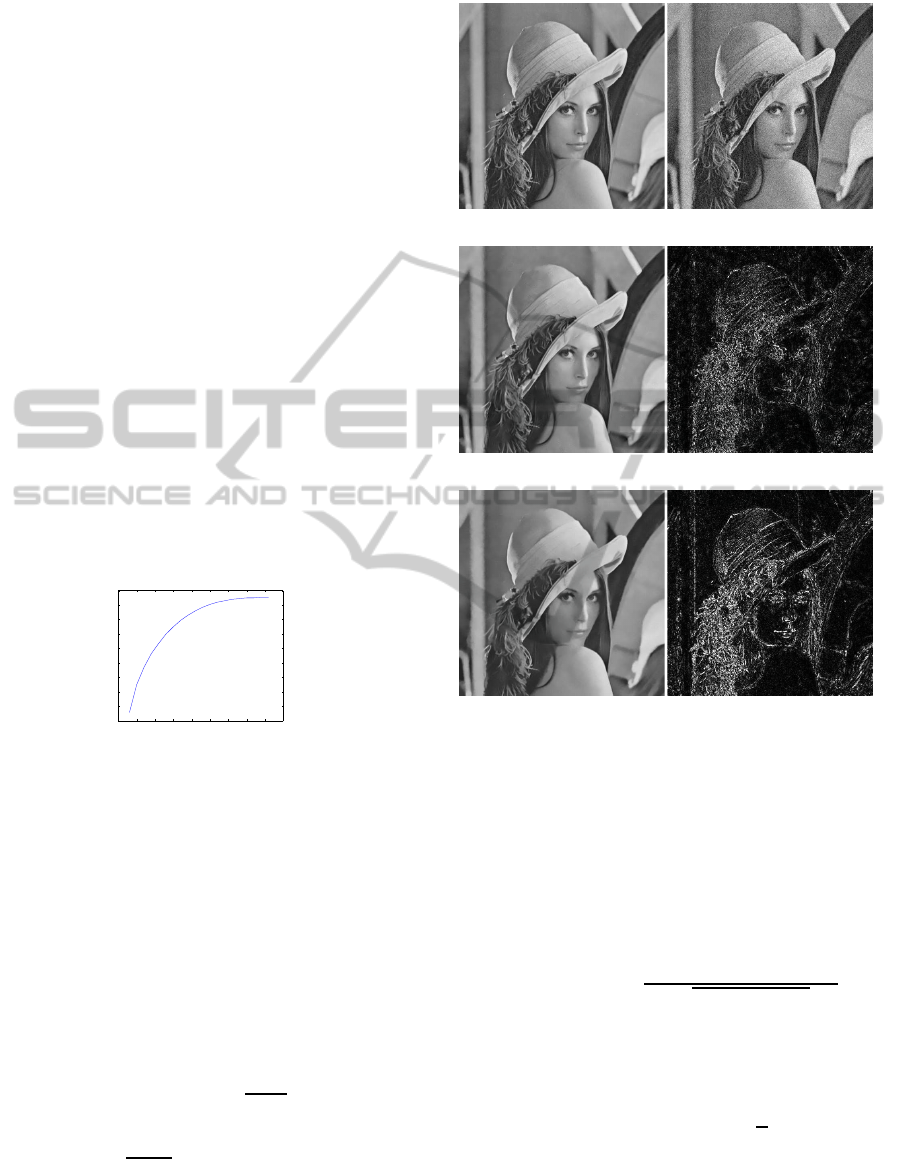
(a) Original image ”Lena”. (b) Noisy image with σ = 20
PSNR = 22.11db.
(c) Restored with OWF. (d) Square error with OWF
PSNR= 32.68db.
(e) Restored with NLMF. (f) Square error with NLMF
PSNR= 31.51db.
Figure 2: Results of denoising ”Lena” 512 ×512 image.
Comparing (d) and (f) we see that the Optimal Weights Fil-
ter (OWF) captures more details than the Non-Local Means
Filter (NLMF).
In the simulations, we sometimes use the
smoothed version of the estimate of brightness varia-
tion d
K
(Y
x,η
,Y
x
0
,η
) instead of the non smoothed one
d (Y
x,η
,Y
x
0
,η
), defined by
d
K
(Y
x,η
,Y
x
0
,η
) =
kK(y) ·(Y
x,η
−Y
x
0
,η
)k
2
q
∑
y
′
∈U
x
0
,η
K(y
′
)
,
where K(y) are some weights defined on U
x
0
,η
.
The corresponding estimate of brightness variation
ρ
f,x
0
(x) is given by
b
ρ
K,x
0
(x) =

d
K
(Y
x,η
,Y
x
0
,η
) −
√
2σ

+
. (19)
With the rectangular kernel
K
r
(y) =

1, y ∈ U
x
0
,η
,
0, otherwise,
(20)
A NEW APPROACH FOR DENOISING IMAGES BASED ON WEIGHTS OPTIMIZATION
115

Table 1: Performance of denoising algorithms when applied to test noisy (WGN) images.
Images Lena Barbara Boat House Peppers
Sizes 512×512 512×512 512×512 256×256 256×256
σ Method PSNR PSNR PSNR PSNR PSNR
Our method(M = 13×13,m = 27×27) 33.93db 32.31db 31.64db 34.09db 31.93db
(Buades et al., 2005) 32.72db 31.67db 30.39db 33.82db 30.97db
15 (Foi et al., 2004) 32.72db 29.61db 30.93db 33.18db 31.78db
(Roth and Black, 2009) 33.29db 30.16db 31.27db 33.55db 32.06db
(Hirakawa and Parks, 2006) 33.97db 32.55db 31.59db 33.82db 31.61db
(Kervrann and Boulanger, 2008) 33.70db 31.80db 31.44db 34.08db 32.13db
(Hammond and Simoncelli, 2008) 34.04db 32.25db 31.72db 33.72db 31.82db
(Aharon et al., 2006) 33.71db 32.41db 31.77db 34.25db 32.20db
(Dabov et al., 2007) 34.27db 33.00db 32.14db 34.94db 32.70db
Our method(M = 13×13,m = 27×27) 32.68db 31.04db 30.30db 32.83db 30.61db
(Buades et al., 2005) 31.51db 30.38db 29.32db 32.51db 29.73db
20 (Foi et al., 2004) 31.43db 27.90db 39.61db 31.84db 30.30db
(Roth and Black, 2009) 31.89db 28.28db 29.86db 32.29db 30.47db
(Hirakawa and Parks, 2006) 32.69db 31.06db 30.25db 32.58db 30.21db
(Kervrann and Boulanger, 2008) 32.64db 30.37db 30.12db 32.90db 30.59db
(Hammond and Simoncelli, 2008) 32.81db 30.76db 30.41db 32.52db 30.40db
(Aharon et al., 2006) 32.39db 30.84db 30.39db 33.10db 30.80db
(Dabov et al., 2007) 33.05db 31.78db 30.88db 33.77db 31.29db
Our method(M = 13×13,m = 27×27) 31.59db 29.92db 29.16db 31.95db 29.40db
(Buades et al., 2005) 30.36db 29.19db 28.38db 31.16db 28.60db
25 (Foi et al., 2004) 30.43db 26.62db 28.60db 30.75db 29.16db
(Roth and Black, 2009) 30.57db 26.84db 28.57db 31.05db 29.17db
(Hirakawa and Parks, 2006) 31.69db 29.89db 29.21db 31.60db 29.06db
(Kervrann and Boulanger, 2008) 31.73db 29.24db 29.20db 32.22db 29.73db
(Hammond and Simoncelli, 2008) 31.83db 29.58db 29.40db 31.54db 29.29db
(Aharon et al., 2006) 31.36db 29.58db 29.32db 32.07db 29.67db
(Dabov et al., 2007) 32.08db 30.72db 29.91db 32.86db 30.16db
we obtain exactly the distance d (Y
x,η
,Y
x
0
,η
) and the
filter described in Section 2. Other smoothing kernels
K(y) used in the simulations are the Gaussian kernel
K
g
(y) = exp

−
N
2
ky−x
0
k
2
2
2h
g

, (21)
where h
g
is the bandwidth parameter, and the follow-
ing kernel: for y ∈ U
x
0
,η
,
K
0
(y) =
Nη
∑
k=max(1, j)
1
(2k+ 1)
2
(22)
if ky−x
0
k
∞
=
j
N
for some j ∈ {0, 1,··· ,Nη}.
The best numerical results are obtained using
K(y) = K
0
(y) in the definition of
b
ρ
K,x
0
. The values
m = 27×27 and M = 13×13 are appropriate in most
cases and a smaller data patch size m can be consid-
ered for processing piecewise smooth images. The
comparison with several filters is given in Table 1.
The PSNR values show that our approach is as good
as more sophisticated methods, like (Hirakawa and
Parks, 2006; Kervrann and Boulanger, 2008; Ham-
mond and Simoncelli, 2008; Aharon et al., 2006), and
is better than the filters proposed in (Foi et al., 2004;
Roth and Black, 2009). Furthermore, our method is
as simple as the Non-Local Means Filter and, with
K(y) = K
0
(y), has only two parameters M and m
which are the sizes of data patches and search win-
dows. The proposed approach gives a denoising qual-
ity which is competitivewith that of the recent method
BM3D (Dabov et al., 2007).
The behavior of the PSNR in function of the size
m of data patches is displayed in Figure 1 for ”Lena”
image. We fix M = 13×13. For σ = 20, Figure 1 il-
lustrates that the PSNR value increases as m varies be-
tween 3×3 and 41×41 (for which PSNR= 32.71db),
and that it just changes slightly when m is sufficiently
large (e.g. PSNR= 32.68db when m = 27 ×27).
In our experimental results (cf. Table 1) we prefer
m = 27 ×27 as the choice m = 41 ×41 is computa-
tionally expensive.
The potential of the estimation method is illus-
trated with the 512×512 image ”Lena” (Figure 2(a))
corrupted by an additivewhite Gaussian noise (Figure
2(b), PSNR = 22.10db, σ = 20). We used the kernel
K
0
(y) for computing the estimated brightness varia-
tion function
b
ρ
K,x
0
, which corresponds to the Opti-
mal Weights Filter as defined in Section 2. In Figure
2(c), we can see that the noise is reduced in a natural
manner and significant geometric features, fine tex-
VISAPP 2012 - International Conference on Computer Vision Theory and Applications
116

tures, and original contrasts are visually well recov-
ered with no undesirable artifacts (PSNR= 32.68db
for ”Lena”). To better appreciate the accuracy of the
restoration process, the square of the difference be-
tween the original image and the recovered image is
shown in Figure 2(d), where the dark values corre-
spond to a high-confidence estimate. As expected,
pixels with a low level of confidence are located in
the neighborhood of image discontinuities. For com-
parison, we show the image denoised by Non-Local
Means Filter in Figures 2(e),(f). The overall visual
impression and the numerical results are improvedus-
ing our algorithm.
The Optimal Weights Filter seems to provide a
feasible and rational method to detect automatically
the details of images and take the proper weights for
every possible geometric configuration of the image.
The distribution of the weights inside the search win-
dow U
x
0
,h
depends on the estimated brightness vari-
ation function
b
ρ
K,x
0
(x), x ∈ U
x
0
,h
. If the estimated
brightness variation
b
ρ
K,x
0
(x) is less than ba (see Theo-
rem 1), the similarity between patches is measured by
a linear decreasing function of
b
ρ
K,x
0
(x); otherwise it
is zero. Thus ba acts as an automatic threshold.
4 CONCLUSIONS
We have proposed a new filter to remove Gaus-
sian noise, based on optimization of weights in the
weighted means approach. Our analysis shows that
a triangular kernel is preferred rather then the Gaus-
sian kernel. The proposed filter improves the usual
Non-Local Means Filter both numerically and visu-
ally in denoising performance; it also has the advan-
tage to be adaptive in the sense that it calculates au-
tomatically the good bandwidth of the triangular ker-
nel (while in the Non-Local Means Filter the choice
of the bandwidth parameter in the Gaussian kernel is
delicate). We hope that the optimal weights that we
deduced can also bring similar improvements for re-
cently developed algorithms where the basic idea of
the Non-Local means filter is used.
ACKNOWLEDGEMENTS
The authors are grateful to the reviewers for helpful
comments and remarks. The work has been partially
supported by the National Natural Science Founda-
tion of China, Grant No. 11101039 and Grant No.
11171044.
REFERENCES
Aharon, M., Elad, M., and Bruckstein, A. (2006). rmk-
svd: An algorithm for designing overcomplete dictio-
naries for sparse representation. IEEE Trans. Signal
Process., 54(11):4311–4322.
Buades, A., Coll, B., Morel, J., et al. (2005). A re-
view of image denoising algorithms, with a new one.
SIAM Journal on Multiscale Modeling and Simula-
tion, 4(2):490–530.
Buades, T., Lou, Y., Morel, J., and Tang, Z. (2009). A note
on multi-image denoising. In Int. workshop on Local
and Non-Local Approximation in Image Processing,
pages 1–15.
Dabov, K., Foi, A., Katkovnik, V., and Egiazarian, K.
(2007). Image denoising by sparse 3-D transform-
domain collaborative filtering. IEEE Trans. Image
Process., 16(8):2080–2095.
Donoho, D. and Johnstone, J. (1994). Ideal spatial adapta-
tion by wavelet shrinkage. Biometrika, 81(3):425.
Foi, A., Katkovnik, V., Egiazarian, K., and Astola, J.
(2004). A novel anisotropic local polynomial estima-
tor based on directional multiscale optimizations . In
Proc. 6th IMA int. conf. math. in signal processing,
pages 79–82.
Hammond, D. and Simoncelli, E. (2008). Image modeling
and denoising with orientation-adapted gaussian scale
mixtures. IEEE Trans. Image Process., 17(11):2089–
2101.
Hirakawa, K. and Parks, T. (2006). Image denoising us-
ing total least squares. IEEE Trans. Image Process.,
15(9):2730–2742.
Katkovnik, V., Foi, A., Egiazarian, K., and Astola, J.
(2010). From local kernel to nonlocal multiple-model
image denoising. Int. J. Comput. Vis., 86(1):1–32.
Kervrann, C. and Boulanger, J. (2008). Local adaptivity
to variable smoothness for exemplar-based image reg-
ularization and representation. Int. J. Comput. Vis.,
79(1):45–69.
Lou, Y., Zhang, X., Osher, S., and Bertozzi, A. (2010). Im-
age recovery via nonlocal operators. J. Sci. Comput.,
42(2):185–197.
Nazin, A., Roll, J., Ljung, L., and Grama, I. (2008). Direct
weight optimization in statistical estimation and sys-
tem identification. System Identification and Control
Problems (SICPRO08), Moscow.
Polzehl, J. and Spokoiny, V. (2006). Propagation-separation
approach for local likelihood estimation. Probab. The-
ory Rel. Fields, 135(3):335–362.
Roth, S. and Black, M. (2009). Fields of experts. Int. J.
Comput. Vision, 82(2):205–229.
Sacks, J. and Ylvisaker, D. (1978). Linear estimation for
approximately linear models. Ann. Stat., 6(5):1122–
1137.
Tomasi, C. and Manduchi, R. (1998). Bilateral filtering for
gray and color images. In Proc. Int. Conf. Computer
Vision, pages 839–846.
Yaroslavsky, L. P. (1985). Digital picture processing. An
introduction. In Springer-Verlag, Berlin.
A NEW APPROACH FOR DENOISING IMAGES BASED ON WEIGHTS OPTIMIZATION
117