
STREAM VOLUME PREDICTION IN TWITTER WITH
ARTIFICIAL NEURAL NETWORKS
Gabriela Dominguez
1
, Juan Zamora
1
, Miguel Guevara
1,3
, H
´
ector Allende
1
and Rodrigo Salas
2
1
Departamento de Inform
´
atica, Universidad T
´
ecnica Federico Santa Mar
´
ıa, Valpara
´
ıso, Chile
2
Departamento de Ingenier
´
ıa Biom
´
edica, Universidad de Valpara
´
ıso, Valpara
´
ıso, Chile
3
Departamento de Computaci
´
on e Inform
´
atica, Universidad de Playa Ancha, Valpara
´
ıso, Chile
Keywords:
Twitter analysis, Stream volume prediction, Artificial neural networks, Time series forecasting.
Abstract:
Twitter is one of the most important social network, where extracting useful information is of paramount im-
portance to many application areas. Many works to date have tried to mine this information by taking the
network structure, language itself or even by searching for a pattern in the words employed by the users. Any-
way, a simple idea that might be useful for every challenging mining task - and that at out knowledge has
not been tackled yet - consists of predicting the amount of messages (stream volume) that will be emitted in
some specific time span. In this work, by using almost 180k messages collected in a period of one week, a
preliminary analysis of the temporal structure of the stream volume in Twitter is made. The expected contri-
bution consists of a model based on artificial neural networks to predict the amount of posts in a specific time
window, which regards the past history and the daily behavior of the network in terms of the emission rate of
the message stream.
1 INTRODUCTION
Twitter has become one of the main communication
medias on the Internet. Users employ this media to
share ideas, news or simply feelings about anything,
producing in this way a valuable footprint about what
is happening at every second and what people think
or feel about it. Nowadays Twitter has become one
of the most popular microblogging services, having
hundreds of millions of messages posted everyday
by more than 50M of users. In Twitter, users post
short messages with a 140 characters length at most
- which are called tweets - commenting about their
thoughts, feelings, recent actions or even discussions
about recent news. Every posted message has asso-
ciated its creation timestamp, the message content,
some user information and also georeferential infor-
mation if there is any.
The massive information content generated in
Twitter has become an interesting source of research
and application. Briefly, some areas and works where
the reader could find a more detailed insight are:
Event detection (Mathioudakis and Koudas, 2010;
Petrovic et al., 2010; Lee et al., 2011), Credibil-
ity Analysis (Mendoza et al., 2010; Castillo et al.,
2011) and Marketing in Social Networks (Domingos,
2005; Banerjee et al., 2010). The high frequency
generation of the data poses important challenges in
terms of storage and processing, given the inherent
online characteristic of this context. It is in this sense
that the stream volume would be a useful informa-
tion for every task of the aforementioned, specially
those tasks that involve important computation pro-
cesses executed in an online fashion.
Time series analysis over streaming data probably
dates back to (Datar et al., 2002), where the authors
propose the sliding window model for computation in
data streams and also tackle the problem of maintain-
ing aggregates statistics of a data stream using this ap-
proach. Several works have follow this path for com-
puting aggregate estimates over streaming data (Zhu
and Shasha, 2002; Guha et al., 2006; Lee and Ting,
2006; Pan et al., 2010), although at our knowledge
no one pointed out to twitter or social network data.
Moreover, the main focus of current works consisted
in enabling the support of selected queries over the
stream instead of the prediction task.
The aim of this preliminary work is to study the
feasibility of forecasting the stream volume of tweets
in certain time span. To accomplish this task we pro-
488
Dominguez G., Zamora J., Guevara M., Allende H. and Salas R. (2012).
STREAM VOLUME PREDICTION IN TWITTER WITH ARTIFICIAL NEURAL NETWORKS.
In Proceedings of the 1st International Conference on Pattern Recognition Applications and Methods, pages 488-493
DOI: 10.5220/0003837004880493
Copyright
c
SciTePress

pose to model the streaming data as an nonlinear au-
toregressive time series (NAR) by using a semipara-
metric model based on a well-known multilayer per-
ceptron. This model will considers the daily behavior
of the stream and allows a parametric prediction hori-
zon. Then, the main goal pursued is to demonstrate
that the temporal structure of the data might be useful
for stream volume prediction regarding its seasonal
behavior. Spite of the simplicity of the idea, we think
that the stream volume prediction using non-linear
models without considering expensive computations
such as fourier or wavelet synopsis, text or network
analysis in data, may fit quite well in the steaming en-
vironment.
This work is organized as follows. In next sec-
tion we deliver the fundamental concepts related to
non-linear time series forecasting with artificial neu-
ral networks. In section 3 we stipulate the proposed
methodology to be able to predict the stream volume.
In section 4 we show preliminary results related to
test the artificial neural network models with different
configurations for the input structure. Finally, some
concluding remarks and future work are given in the
last section.
2 BACKGROUND
2.1 Artificial Neural Networks
Artificial Neural Networks (ANN) have received a
great deal of attention in many fields of engineering
and science. Inspired by the study of brain architec-
ture, ANN represent a class of non-linear models ca-
pable of learning from data. The essential features of
an ANN are the basic processing elements referred to
as neurons or nodes; the network architecture describ-
ing the connections between nodes; and the training
algorithm used to estimate values of the network pa-
rameters.
Artificial Neural Networks (ANN) are seen by
researches as either highly parameterized models or
semiparametric structures. ANN can be considered
as hypotheses of the parametric form h(·; w), where
the hypothesis h is indexed by the parameter w. The
learning process consists in estimating the value of the
vector of parameters w in order to adapt the learner h
to perform a particular task.
The Multilayer Perceptron (MP) is the most pop-
ular and widely known artificial neural network. In
this network, the information is propagated in only
one direction, forward, from the input nodes, through
the hidden nodes (if any) and to the output nodes. Fig-
ure 1 illustrates the architecture of this artificial neu-
Figure 1: Network architecture of the Multilayer Percep-
tron.
ral network with one hidden layer. Furthermore, this
model has been deeply studied and several of its prop-
erties have been analyzed. One of the most important
theorem is about its universal approximation capabil-
ity (see (Hornik et al., 1989) for details), and this the-
orem states that every bounded continuous function
with bounded support can be approximated arbitrar-
ily closely by a multi-layer perceptron by selecting
enough but a finite number of hidden neurons with
appropriate transfer function.
The non-linear function h(x, w) represents the out-
put of the multilayer perceptron, where x is the input
signal and w being its parameter vector. For a three
layer MP (one hidden layer), the output computation
is given by the following equation
g(x, w) = f
2
λ
∑
j=1
w
[2]
k j
f
1
d
∑
i=1
w
[1]
ji
x
i
+ w
[1]
j0
!
+ w
[2]
k0
!
(1)
where λ is the number of hidden neurons. An im-
portant factor in the specification of neural models is
the choice of the transfer function, these can be any
non-linear function as long as they are continuous,
bounded and differentiable. The transfer function of
the hidden neurons f
1
(·) should be nonlinear while
for the output neurons the function f
2
(·) could be a
linear or nonlinear function.
The MP learns the mapping between the input
space X to the output space Y by adjusting the
connection strengths between the neurons w called
weights. Several techniques have been created to esti-
mate the weights, where the most popular is the back-
propagation learning algorithm, also known as gen-
eralized delta rule, popularized by (Rumelhart et al.,
1986).
2.2 Non-linear Time Series Prediction
The statistical approach to forecasting involves the
construction of stochastic models to predict the value
of an observation x
t
using previous observations. This
is often accomplished using linear stochastic differ-
STREAM VOLUME PREDICTION IN TWITTER WITH ARTIFICIAL NEURAL NETWORKS
489

2000 4000 6000 8000
20
40
60
80
100
Time (minutes)
Number of Tweets
(a) 1 minute.
500 1000 1500
100
200
300
400
500
Time (5 minutes)
Number of Tweets
(b) 5 minutes.
200 400 600 800
100
200
300
400
500
600
700
800
Time (10 minutes)
Number of Tweets
(c) 10 minutes.
100 200 300 400 500
200
400
600
800
1000
Time (15 minutes)
Number of Tweets
(d) 15 minutes.
20 40 60 80 100 120 140
500
1000
1500
2000
2500
3000
Time (hour)
Number of Tweets
(e) 1 hour.
Figure 2: Aggregated time series of the Chilean tweets stream sampled between 20th through 26th of July 2011. The selected
windows size are (a) 1 minute, (b) 5 minutes, (c) 10 minutes, (d) 15 minutes, and, (d) 1 hour.
ence equation models. By far, the most important
class of such models is the linear autoregressive in-
tegrate moving average (ARIMA) model.
An important class of Non-linear Time Series
models is that of non-linear Autoregressive mo-
dels (NAR) which is a generalization of the lin-
ear autoregressive (AR) model to the non-linear
case. A NAR model obeys the equation x
t
=
h(x
t−1
, x
t−2
, ...., x
t−p
) + ε
t
, where h is an un-
known smooth non-linear function and ε
t
is white
noise, and it is assumed that E[ε
t
|x
t−1
, x
t−2
, ...] =
0. In this case the conditional mean predic-
tor based on the infinite past observation is ˆx
t
=
E[h(x
t−1
, x
t−2
, ...)|x
t−1
, x
t−2
, ...], with the following
initial conditions ˆx
0
= ˆx
−1
= ... = 0.
Artificial Neural Networks have been successfully
applied as a NAR model in time series forecasting.
Refer to the work of (Balestrassi et al., 2009) for fur-
ther details.
3 METHODOLOGY
3.1 Data Collection and Processing
In this work we obtain preliminary results with a lit-
tle collection of Tweets obtained in a region encom-
passing the central part of Chile during the period of
time covered between the 20th and 26th of July, 2011,
where the amount of post sum up to 171.991 tweets
obtained in a time span of almost 6 days (8488 min-
utes). In previous work, we have characterized the
tendency based on the most frequent terms, number
of tweets per user, amount of link references, among
others descriptive results.
The collected messages was accomplished by us-
ing the streamming API of Twitter using the Python
language, together with the Json (module to process
data in JSON format) toolkit. The collected Tweets
messages are in a JSON format (JavaScript Object
Notation) that is a lightweight data-interchange for-
mat with the characteristic that it is easy to parse
and generate. With Json, the tweets messages were
exported to several formats as XML and TXT. The
streamming API allows to access in near-realtime to a
random sub-set of publicly available Twitter data, we
configured the API with the statuses/sample method
to have a feed of 1% of real volume of Tweets, this
mode is called Spritzer.
The Tweet structure has a timestamp at the cre-
ated at field. We have sorted the post according this
timestamp, and then we proceeded to aggregate the
information by counting the number of Tweets gen-
erated in a time-window defined by the user. In this
work we have selected the windows of size 1-minute,
5-minutes, 10-minutes, 15-minutes and 1-hour. Fig-
ure 2 graphically shows the summary of the aggre-
gated time series with different windows size.
ICPRAM 2012 - International Conference on Pattern Recognition Applications and Methods
490
3.2 Stream Volume Forecasting
To forecast the volume of messages we model the
stochastic process as a non-linear autoregressive
(NAR) time series. However, a difficult issue in time
series forecasting is the structural identification of the
model, where the relevant lags are hard to find. How-
ever in this preliminary work we exhaustively test
some configurations with the aim of knowing if we
are able to make one step prediction based on past
information. The selected configurations are shown
in table 1, where configurations C1, C2 and C3 were
tested for all windows size. On the other hand the
configurations C4, C5, C6, C7 and C8 wer tested for
the windows of size 1-minute, 5-minutes, 10-minutes,
15-minutes, 1-hour respectively, in order to elucidate
if there exist any seasonal contribution.
The multilayer perceptron with three layers was
applied to model de NAR process. The architecture
of the neural network consists in three layers of neu-
rons, where the number of input neurons depends on
the number of lags of each selected configuration, the
number of output neurons was set in one (1-step pre-
diction), and we arbitrarily decided to test with two
hidden neurons to maintain a low complexity of the
model. We selected the log sigmoid transfer function,
f
1
(z) =
1
1 + e
−z
for the hidden neurons and the linear transfer func-
tion, f
2
(z) = z, for the output neurons. The parame-
ters were estimated with the training function that up-
dates weight and bias values according to Levenberg-
Marquardt optimization. For this study we have used
the Neural Nework toolbox of Matlab.
4 RESULTS
For the experiments, we have partitioned the data
sets, structured according to the selected configura-
tions given in table 1, in three sets: Training (70% of
the data), Validation (15% of the data) and Test (15%
of the data). In this section we report the best perfor-
mance result obtained after 5 runs for each model. We
have computed the mean square error (MSE)
MSE =
1
n
n
∑
i=1
(y
i
− ˆy
i
)
2
(2)
and the correlation coefficient (R)
R =
∑
n
i=1
(y
i
−Y )( ˆy
i
− P)
q
∑
n
i=1
(y
i
−Y )
2
q
∑
n
i=1
( ˆy
i
− P)
2
(3)
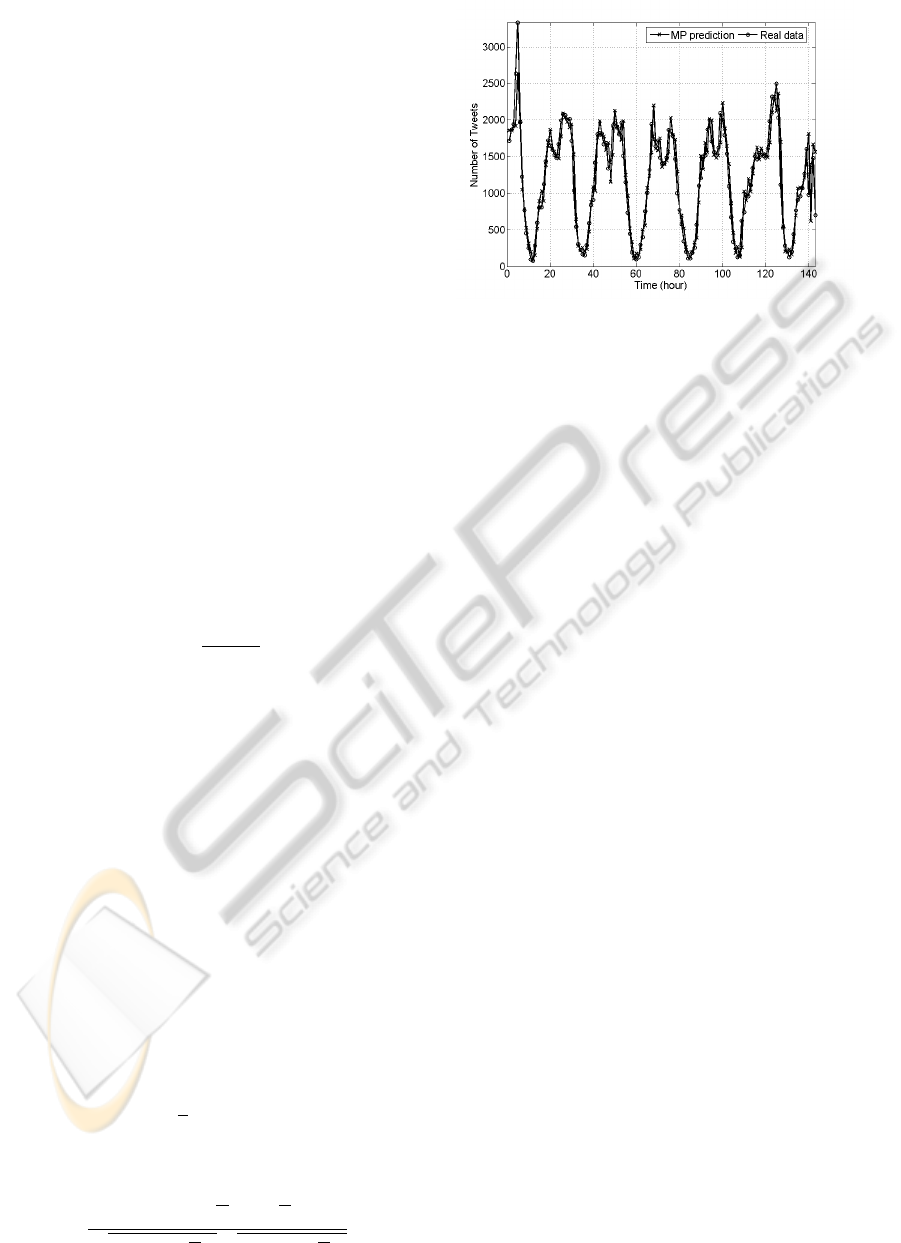
Figure 3: Multilayer perceptron prediction with configura-
tion 2 for the 1-hour time window.
for the predictions in the Test set. Tables 2(a), 2(b),
2(c), 2(d) and 2(e) show the performance of the MP
and an autoregressive model (baseline) for the stream
volume prediction task with different window size
and by testing several configurations (shown in ta-
ble 1). In bold are highlighted the best results for
each time-window (Two decimals approximation was
made over the results).
In all the simulations we have a correlation coeffi-
cient higher than 80% and with a relatively low error,
with this results we have shown that it is feasible to
forecast the stream volume with the multilayer per-
ceptron. Although the identification of the best lags
configuration remains as an open issue, the perfor-
mance are similar among them. We were not able to
detect the seasonal component in almost all cases with
the exception of the 10-minutes and 15-minutes win-
dows size. In general the best results were obtained
for the third configuration that it is characterized by
containing more lags with recently past information
than the other configurations. Figure 3 qualitatively
shows the prediction performance of the best resulting
configuration for the multilayer perceptron in model-
ing the stream volume with a 1-hour time-window.
5 CONCLUSIONS
In this paper we were able to give a solution to
the problem of stream volume prediction in Twitter,
where a non-linear autoregressive time series model,
based on artificial neural networks, is used to predict
the amount of posts in a specific time window. This
model will considers the recently past history together
with a seasonal component to improve the prediction
of the amount of messages that will arrive during the
upcoming time period.
Furthermore, regarding the performance values pre-
STREAM VOLUME PREDICTION IN TWITTER WITH ARTIFICIAL NEURAL NETWORKS
491

Table 1: Selected configurations of the autoregressive structure of the time series data.
(a)
Configuration Lags
C1 x
t−1
C2 x
t−1
, x
t−2
C3 x
t−1
, x
t−2
, , x
t−3
C4 x
t−1
, x
t−1440
, x
t−1441
(b)
Configuration Lags
C5 x
t−1
, x
t−288
, x
t−289
C6 x
t−1
, x
t−144
, x
t−145
C7 x
t−1
, x
t−96
, x
t−97
C8 x
t−1
, x
t−24
, x
t−25
Table 2: Summary of the results for the prediction performance obtained by the MP for the 1-minute (table 2(a)), 5-minutes
(table 2(b)), 10-minutes (table 2(c)), 15-minutes (table 2(d)) and 1-hour (table 2(e)) time window.
(a)
ANN AR
Config. MSE R MSE R
C1 30.80 0.86 38.42 0.86
C2 27.10 0.89 31.15 0.89
C3 24.07 0.90 28.58 0.90
C4 35.60 0.88 33.34 0.88
(b)
ANN AR
Config. MSE R MSE R
C1 417.14 0.92 571.48 0.92
C2 317.48 0.94 464.10 0.93
C3 271.44 0.94 434.57 0.94
C5 412.46 0.94 394.42 0.94
(c)
ANN AR
Config. MSE R MSE R
C1 2764 0.86 3802.65 0.85
C2 2167 0.88 3647.86 0.86
C3 1976 0.89 3504.11 0.86
C6 2264 0.92 2017.84 0.92
(d)
ANN AR
Config. MSE R MSE R
C1 11605 0.87 8044.59 0.86
C2 12455 0.86 7571.96 0.87
C3 11791 0.90 7346.80 0.87
C7 4154 0.88 5885.25 0.90
(e)
ANN AR
Config. MSE R MSE R
C1 53628 0.90 93505.67 0.89
C2 28545 0.94 67112.10 0.93
C3 30043 0.94 66873.07 0.93
C8 79056 0.92 38874.10 0.95
sented in table 2, it results interesting to notice that
even when the R achieved by both models under eval-
uation are comparable in every time window, the MSE
value attained by the MP is substantially lower. This
observation may suggests that the last mentioned mo-
del could be an acceptable choice for data contain-
ing outliers and high frequency observations, com-
mon features found in the streaming context. Any-
way, a more thorough validation is required given the
random initialization of the ANN. Finally, by observ-
ing fig. 2, a change in the shape pattern presented by
the first two plots is noticed in comparison to the two
next plots. After that, the first shape pattern is repited
for the 1-hour plot. More data is needed to outline a
conclusion about this point.
Future works are needed in order to determine the
best lags that elucidate the time-structure of the au-
toregressive model. Several applications in Twitter
analysis can be supported by our proposed model as
for example event detection. Due to the noise and the
presence of outliers in the data, in specific at lower
levels of aggregation, robust procedures are needed to
better estimate the model parameters and enhance the
prediction. We are planing to collect data for a longer
period of time and maybe by considering a higher en-
compassing spatial region in order to better validate
the proposed model.
ACKNOWLEDGEMENTS
The work of H
´
ector Allende was supported by the re-
search grant FONDECYT 1110854. The work of Ro-
drigo Salas was supported by the research grant DIUV
37/2008. The work of Juan Zamora has been partially
supported by the research grant FONDEF-CONICYT
D09I1185.
ICPRAM 2012 - International Conference on Pattern Recognition Applications and Methods
492

REFERENCES
Balestrassi, P., Popova, E., Paiva, A., and Marangon-Lima,
J. (2009). Design of experiments on neural network’s
training for nonlinear time series forecasting. Neuro-
computing, 72:1160–1178.
Banerjee, S., Al-Qaheri, H., and Hassanien, A. E. (2010).
Mining social networks for viral marketing using
fuzzy logic. In Mathematical/Analytical Modelling
and Computer Simulation (AMS), 2010 Fourth Asia
International Conference on, pages 24 –28.
Castillo, C., Mendoza, M., and Poblete, B. (2011). Informa-
tion credibility on twitter. In Proceedings of the 20th
international conference on World wide web, WWW
’11, pages 675–684, New York, NY, USA. ACM.
Datar, M., Gionis, A., Indyk, P., and Motwani, R. (2002).
Maintaining stream statistics over sliding windows:
(extended abstract). In Proceedings of the thir-
teenth annual ACM-SIAM symposium on Discrete al-
gorithms, SODA ’02, pages 635–644, Philadelphia,
PA, USA. Society for Industrial and Applied Math-
ematics.
Domingos, P. (2005). Mining social networks for viral mar-
keting. IEEE Intelligent Systems, 20(1):80–82.
Guha, S., Koudas, N., and Shim, K. (2006). Approximation
and streaming algorithms for histogram construction
problems. ACM Trans. Database Syst., 31:396–438.
Hornik, K., Stinchcombe, M., and White, H. (1989). Multi-
layer feedforward networks are universal approxima-
tors. Neural Networks, 2:359–366.
Lee, C.-H., Wu, C.-H., and Chien, T.-F. (2011). BursT:
A dynamic term weighting scheme for mining mi-
croblogging messages. In Liu, D., Zhang, H., Polycar-
pou, M., Alippi, C., and He, H., editors, Advances in
Neural Networks ISNN 2011, volume 6677 of Lecture
Notes in Computer Science, pages 548–557. Springer
Berlin / Heidelberg.
Lee, L. K. and Ting, H. F. (2006). Maintaining significant
stream statistics over sliding windows. In Proceedings
of the seventeenth annual ACM-SIAM symposium on
Discrete algorithm, SODA ’06, pages 724–732, New
York, NY, USA. ACM.
Mathioudakis, M. and Koudas, N. (2010). Twittermonitor:
trend detection over the twitter stream. In Proceedings
of the 2010 international conference on Management
of data, SIGMOD ’10, pages 1155–1158, New York,
NY, USA. ACM.
Mendoza, M., Poblete, B., and Castillo, C. (2010). Twitter
under crisis: can we trust what we rt? In Proceed-
ings of the First Workshop on Social Media Analytics,
SOMA ’10, pages 71–79, New York, NY, USA. ACM.
Pan, B., Demiryurek, U., Banaei-Kashani, F., and Shahabi,
C. (2010). Spatiotemporal summarization of traffic
data streams. In Proceedings of the ACM SIGSPATIAL
International Workshop on GeoStreaming, IWGS ’10,
pages 4–10, New York, NY, USA. ACM.
Petrovic, S., Osborne, M., and Lavrenko, V. (2010). Stream-
ing first story detection with application to twitter.
In HLT-NAACL, pages 181–189. The Association for
Computational Linguistics.
Rumelhart, D., Hinton, G., and William, R. (1986). Learn-
ing internal representation by back-propagation er-
rors. Nature, 323:533–536.
Zhu, Y. and Shasha, D. (2002). Statstream: Statistical mon-
itoring of thousands of data streams in real time. In
VLDB, pages 358–369. Morgan Kaufmann.
STREAM VOLUME PREDICTION IN TWITTER WITH ARTIFICIAL NEURAL NETWORKS
493
