
COPING WITH LONG TERM MODEL RISK IN MARKET RISK
MODELS
Manuela Spangler
1
and Ralf Werner
2
1
Deutsche Pfandbriefbank AG, Risk Models & Analytics, Freisinger Str. 5, 85716 Unterschleissheim, Germany
2
Hochschule M¨unchen, Fakult¨at f¨ur Informatik und Mathematik, Lothstr. 64, 80335 M¨unchen, Germany
Keywords:
Model risk, Risk management.
Abstract:
The recent financial crisis has shown that most market risk models – even if they deliver sufficiently accurate
risk figures over short time horizons – are not able to provide reliable forecasts for risk figures over longer time
horizons like three, twelve or 36 months, which are the basis for both limit management and economic capital
planning. As a potential remedy the concept of potential future market risk can be used to deal with such long
term model risks in market risk measurement. Based on a toy example we will outline how this concept can
be applied for new business planning or for limit setting and capital buffer definitions.
1 DEFINITION OF MODEL RISK
In the context of market risk measurement, model risk
is usually understood as the risk that the model used
for market risk measurement is specified wrongly and
does therefore not or not fully capture the risks it was
designed to measure (Jorion, 2007), Section 21.2.6.
In the following, however, we focus on a different
point of view along the lines of (Jorion, 2007), Chap-
ter 9, and thus we need to distinguish between differ-
ent kinds of model risk.
Short Term Model Risk. Short term model risk arises
from the fact that model assumptions may be violated,
which also includes parameter uncertainty (i.e. esti-
mation risk). Taking the example of a delta-normal
VaR model, the linear impact of risk factor changes
on the portfolio value as well as the normal distribu-
tion assumption with constant volatility for risk fac-
tor changes are such assumptions. Short term model
risk is usually an issue for the daily risk measurement
process, see for example (Figlewski, 2003) or (Hen-
dricks, 1996). (Berkowitz and OBrien, 2002) anal-
yse the accuracy of VaR forecasts for banks’ trading
desks based on the models used in practice. There
is vast literature on how short term model risk can
be identified and controlled via back-testing proce-
dures, see e.g. (Kupiec, 1995), (Christoffersen et al.,
2001), (Christoffersen and Pelletier, 2004) or more
recently (Berkowitz et al., 2011); or how it can be
handled via more sophisticated models, see for in-
stance (Kamdem, 2005) for an extension to elliptical
distributions, (Alexander, 2001) for a non-parametric
linear historical or Monte-Carlo VaR or (Bams and
Wielhouwer, 2001) for adjustment factors for estima-
tion risk. (Alexanderand Sarabia, 2011) quantify VaR
model risk and derive an add-on factor for market
risk capital. Similarly, (Kerkhof et al., 2010) derive
an add-on to capital reserves which accounts for VaR
model risk and distinguishes between estimation and
misspecification risk.
Long Term Model Risk. This kind of model risk cov-
ers the risk that the reported daily risk figures change
in an adverse fashion over longer time scales, al-
though the portfolio itself remains unchanged. This
means that even if the risk is reasonably measured
and predicted for small time horizons by the model,
the market risk number might change on a daily basis
and, therefore, cannot be used for longer term plan-
ning. Delta-normal VaR figures, for example, are
highly impacted by (i) changing volatilities and cor-
relations, and (ii) changing portfolio sensitivities. Be-
fore the beginning of the financial crisis, long term
model risk was not considered to be an issue for banks
or financial institutions
1
, as any unwanted shift or in-
crease in VaR figures could be easily countered by
hedging or risk reduction actions. Since the second
half of 2007, however, significant parts of trading
1
As one of a few exceptions, let us mention the exposi-
tions by (Jorion, 2007), Section 9.5 or (Danielsson, 2002),
who point out that VaR figures are volatile and not reliable
in general.
239
Spangler M. and Werner R..
COPING WITH LONG TERM MODEL RISK IN MARKET RISK MODELS.
DOI: 10.5220/0003712902390246
In Proceedings of the 1st International Conference on Operations Research and Enterprise Systems (ICORES-2012), pages 239-246
ISBN: 978-989-8425-97-3
Copyright
c
2012 SCITEPRESS (Science and Technology Publications, Lda.)

portfolios became more and more illiquid, risks could
no longer be hedged adequately, and risk figures in-
creased in an unpredicted fast and threatening fash-
ion. Potential consequences were limit breaches, or in
worst case situations, additional capital requirements
to keep the financial institution solvent. In the follow-
ing, we therefore discuss long term model risk only,
with a special focus on the implications for limit man-
agement and economic capital planning.
As long term model risk is a rather novel issue,
there is not much literature available. (Christoffersen
and Goncalves, 2005) or (Jorion, 1996), who investi-
gate the statistical properties of VaR figures in detail,
propose confidence intervals around VaR estimates to
cover model risk. Their expositions are, however,
mainly centred around short term model risk. To
quantify long term model risk we are more interested
in the extent to which VaR figures may change in fu-
ture. Therefore, we need to take into account potential
future evolutions of market environments. Taking the
ideas by Christoffersen, Goncalves and Jorion further,
this immediately leads to the concept of potential fu-
ture value-at-risk (PFVaR), developed by (Spangler
and Werner, 2010). There, a detailed explanation of
the concept is given together with a specific example
on the computation of the corresponding risk figures.
Here, we briefly recall the main definitions of PFVaR
from (Spangler and Werner, 2010), before we focus
on the application of the concept in risk management.
2 THE CONCEPT OF
POTENTIAL FUTURE
VALUE-AT-RISK
For the proper definition of PFVaR, let us fix a static
portfolio, a reference time t
R
(i.e. today) and let us de-
note the future (random) VaR figure at time t > t
R
with
VaR
α
(t) for a given VaR level α.
2
Similarly to the po-
tential future exposure concept in counterparty credit
risk (see (Pykhtin, 2005) for more details), a few ver-
sions of PFVaR have been introduced by Spangler and
Werner:
• The expected VaR at time T > t
R
is the average of
the potential future VaR at time T:
EVaR
α
(T) := E[VaR
α
(T) | F
t
R
]. (1)
• The peak VaR at time T > t
R
is the maximum VaR
that is expected to occur at time T at a given con-
fidence level (quantile) β ∈ (0, 1):
PVaR
α,β
(T) := q
β
[VaR
α
(T) | F
t
R
]. (2)
2
As the VaR time horizon h is fixed throughout the fol-
lowing, we skip it for notational convenience.
• The maximum peak VaR until time T > t
R
is the
maximum VaR that is expected to occur in [t
R
, T]
at a given confidence level β ∈ (0, 1):
MPVaR
α,β
(T) := q
β
max
t∈[t
R
,T]
[VaR
α
(t) | F
t
R
]
.
(3)
All introduced quantities are conditional on the
information (i.e. the corresponding filtration F
t
R
)
given at the reference time t
R
, which means that
quantiles or expectations calculated at time t
R
only include information available up to time t
R
.
It has to be noted that for a one-to-one relation-
ship of PFVaR and the potential future exposure
concept in counterparty credit risk, the maximum
peak VaR would have to be defined by
MPVaR
α,β
(T) = max
t∈[t
R
,T]
PVaR
α,β
(t)
= max
t∈[t
R
,T]
q
β
(VaR
α
(t) |F
t
R
)
.
In the above definition (3), the order of maximiza-
tion and percentile has been switched as it is more
meaningful for practical applications: the maxi-
mum peak VaR is exceeded by VaR
α
(t) in the pe-
riod [t
R
, T] with a probability of 1− β.
The concept of potential future VaR can be easily gen-
eralized to potential future market risk when replac-
ing VaR by any arbitrary market risk measure. For
the calculation of the PFVaR figures an appropriate
model needs to be specified to project risk figures
forward in time. Analogously to risk modelling, the
choice of the appropriate methodology, i.e. the choice
between historical bootstrapping or Monte Carlo sim-
ulation (e.g. GARCH models or discretized SDEs),
has a strong impact on the resulting figures. Depend-
ing on the purpose and on the time horizon, Span-
gler and Werner suggested to either use a pure and
simplistic historical bootstrapping method similarly
to (Christoffersen and Goncalves, 2005) or, alterna-
tively to use a more sophisticated integrated economic
scenario generator,see (Davidson, 2008), which is es-
pecially designed for projections of the joint evolu-
tion of risk factors over longer time horizons. For the
specific calculation of the PFVaR figures and the con-
crete choice of the model, let us refer to (Spangler and
Werner, 2010).
3 APPLICATIONS OF PFVAR
PFVaR as such represents an add-on to existing mar-
ket risk frameworks without the need to amend a
bank’s current market risk systems. For instance,
ICORES 2012 - 1st International Conference on Operations Research and Enterprise Systems
240

based on the algorithm presented by Spangler and
Werner, a bank’s market risk system can be re-used
to calculate the corresponding PFVaR figures without
much additional effort. The requirements on the com-
putational capabilitites of the market risk (and front
office) system are actually the same as for CVA (coun-
terparty value adjustment) or counterparty credit risk
calculations, which are nowadays already in place for
most banks.
From a management perspective, PFVaR provides
a consistent framework to measure and handle long
term model risk within a bank’s planning and man-
agement processes:
• Taking the expected VaR at certain time horizons
T
1
, .. . ,T
n
yields precise information on how fast
risk will decay on average, especially compared to
traditional time-to-maturity or duration concepts.
The expected VaR not only covers the ageing ef-
fect of the portfolio, but can also account for ex-
pected increases in volatility or correlation. Thus,
the sustainability of hedging activities over longer
time horizons can easily be analyzed based on the
expected VaR.
It is furthermore well-suited for the planning
process, and especially suitable for planning of
new business. In general, new business volumes
should be chosen in such a way that the expected
future risk fits to the overall planning figures for
future time horizons. In such a context, time hori-
zons from one to three years are usually consid-
ered by banks. These longer time horizons there-
fore require the same models for the evolution of
the risk factors as in long term counterparty credit
risk modelling. However, in contrast to scenar-
ios calibrated for counterparty credit risk purposes
based on historical data, the focus on planning
usually requires that the expected risk factor evo-
lution coincides with some best estimate planning
scenario provided by a bank’s strategic planning
department.
• The future VaR distribution, and especially the
peak VaR, provides additional valuable insights
for the limit management process, as for a fixed
portfolio it shows by how much future market risk
figures may fluctuate. To avoid limit breaches due
to changes in volatilities and correlation, these
fluctuations should be taken into account when
setting limits based on reasonable levels of β.
Whereas any new trade should be considered
against limits derived from the expected future
VaR, the size of capital buffers in risk capital plan-
ning should be based on the excess of the peak
VaR against the expected VaR. Then, assuming a
limit breach of the expected VaR limit is not due
to new business or trading activities, the excess
of the risk against the limit can be absorbed by
the additional buffer. Only when this buffer is ex-
hausted, a limit breach is reported.
• Further, economic capital models under going-
concern assumptions do not only need to model
trading losses at some future point in time, but
also need to forecast the future VaR consump-
tion.
3
Given the obvious ambiguity about the
future market risk exposure, the peak VaR pro-
vides guidance on how (a maybe downscaled ver-
sion of) the current portfolio would behave in
a stressed environment as assumed by economic
capital models. Thus, in going-concern economic
capital models, market risk capital should be suf-
ficient to cover both severe losses (i.e. decreases
in market value) plus a stressed market risk level.
Taking the stress test point of view, peak VaR
also represents a good choice for VaR figures
within stress scenarios used in macro-economic
integrated stress tests. The peak VaR therefore
can act as a supplement to usual risk figures, if
β is chosen in accordance to the severity of the
applied stress test.
• Finally, the maximum peak VaR represents the
maximum VaR figure which may be observed in a
stress scenario where markets become completely
illiquid and risks cannot be reduced by hedging
activities. Given the maximum peak VaR, both
the likelihood as well as the amount of a potential
limit breach can be derived, which can, for exam-
ple, be used in contingency planning.
4 EXAMPLE: TWO-FACTOR
DELTA-NORMAL VAR
FRAMEWORK
Let us consider a hypothetical portfolio consisting of
Greek and Spanish floating rate government bonds
with different maturities. Since the portfolio consists
of floating rate bonds only, interest rate risk plays
a minor role and will therefore be neglected in the
following examinations. The remaining details of
the setup are the same as in Spangler and Werner:
for credit spread risk measurement, we use a two-
factor delta-normal VaR approach; credit spread mar-
ket movementsare explained by two credit spread risk
factors (zero spreads) which are assumed to havea flat
3
Under a going-concern point of view, it cannot be
reasonably assumed that all market risks are completely
hedged.
COPING WITH LONG TERM MODEL RISK IN MARKET RISK MODELS
241

2004 2005 2006 2007 2008 2009 2010
−100
0
100
200
300
Time
Spread (bp)
Risk factor time series
10Y Greek spread
10Y Spanish spread
2005 2006 2007 2008 2009 2010
0
50,000
100,000
150,000
Time
VaR
Credit spread risk figures
Total portfolio
Greek subportfolio
Spanish subportfolio
Figure 1: Risk factors and corresponding portfolio credit spread risk figures over time.
term structure that can change over time
4
. As risk fac-
tor proxies we have chosen 10-year asset swap spread
time series for Greek and Spanish government bonds,
cf. Figure 1, upper part. The lower part of Figure 1
shows the historical 1-day 99% credit spread VaR of
the assumed portfolio.
4.1 Portfolio VaR Decomposition
In order to identify the impact of changing volatili-
ties and correlations, changes in risk factor levels and
ageing effects on VaR figures let us consider Figure 2
which shows the decomposition of logarithmic VaR
changes from initial time t
I
to time T according to
(4), decomposed into changes caused by shifts in the
covariance matrixC
t
and changes in the sensitivity S
t
.
ln
VaR
α
(T)
VaR
α
(t
I
)
| {z }
Total impact
=ln
q
S
⊤
T
·C
T
· S
T
q
S
⊤
T
·C
t
I
· S
T
| {z }
Impact of covariance
(4)
+ln
q
S
⊤
T
·C
t
I
· S
T
q
S
⊤
t
I
·C
t
I
· S
t
I
| {z }
Impact of sensitivity
(5)
Although the influence of sensitivities on VaR figures
is considerable – VaR is reduced by up to ≈ 50%
of the original value – the impact of the covariance
4
As rather similar results are obtained if a more general
framework (i.e. varying term structures) is considered, we
focus on this simplified setting for the brevity and clarity of
presentation.
matrix is even stronger: it accounts for a factor
of ≈ 570%. Although the effects tend to cancel
out to a certain extent, a once feasible portfolio
(i.e. within market risk limits) can easily exceed its
limit over time by a large or actually economic capital
threatening amount. For a further analysis, Figure 2
also details the effects of the sensitivities and the
covariance matrix, which shows that for the given
portfolio, ageing dominates level effects. Further,
changes caused by covariance shifts are mainly due
to (Greece) volatilities, not correlation.
Looking at a rolling one-year horizon instead of
the complete VaR history, Figure 3 displays a
rather constant influence of ageing, leading to an
annual risk reduction of about 15% per annum
(VaR
α
(t) ≈ 0.85 · VaR
α
(t − 1Y)) compared to a
maximum increase of 270% over one year caused by
rising volatilities. From Figure 3 it can be seen that
VaR increases steadily from 2007 to 2009 and then
explodes from the beginning of 2009 onwards.
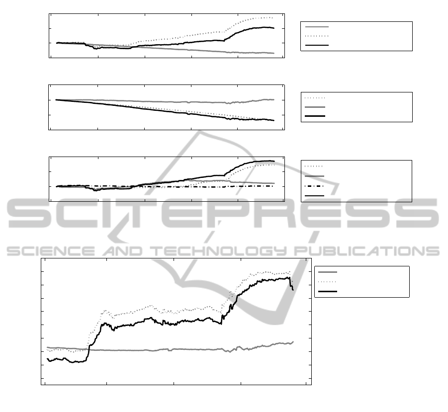
4.2 PFVaR Analysis
To illustrate the concept of PFVaR, Figure 4 shows
a sample of 100 bootstrapped scenarios of length
250 days against the actual historical evolution of the
Spanish credit spread risk factor.
As can be seen from Figure 5 (upper part), the
concept of potential future works well before Septem-
ber 2008.
• The expected VaR shows that VaR reducing age-
ing effects are expected to be compensated by an
increase in volatility (due to the moving estima-
ICORES 2012 - 1st International Conference on Operations Research and Enterprise Systems
242
Impact of sensitivity
Impact of covariance
Total impact
2005 2006 2007 2008 2009 2010
−1
0
1
2
Time
Logarithmic
impact
Decompositon of total impact
2005 2006 2007 2008 2009 2010
−1
−0.5
0
0.5
Decompositon of sensitivity impact
Time
Logarithmic
impact
Impact of aging
Impact of level
Total impact of sensitivity
2005 2006 2007 2008 2009 2010
−1
0
1
2
Decompositon of covariance impact
Time
Logarithmic
impact
Impact of volatility (GR)
Impact of volatility (ES)
Impact of correlation
Total impact of covariance
Figure 2: Impact of sensitivity and covariance parameters on portfolio VaR.
2006 2007 2008 2009 2010
−0.6
−0.4
−0.2
0
0.2
0.4
0.6
0.8
1
Time
Logarithmic Impact
1Y rolling decomposition of total impact
Impact of sensitivity
Impact of covariance
Total impact
Figure 3: Impact of sensitivity and covariance parameters on portfolio VaR over a rolling one-year time horizon.
tion window), resulting in relatively stable VaR
figures on average. The (maximum) peak VaR
gives a reasonable upper bound on VaR, as long
as there is no regime switch in the market.
• Without additional capital, no new business can
be planned for, as the expected VaR remains on
the same level as the initial VaR of January 2008.
This is in contrast to the maturity or duration pro-
file which would have indicated a potential for
new business around 5% to 15%. The gap is
mainly due to increasing volatilities as a very calm
period at the beginning of 2007 is dropped from
the rolling 250-day time window for the historical
data used for VaR calculations.
• While the VaR limit can be fixed at the current
level and no new business is possible, an addi-
tional limit or capital buffer for market risk of
around 30% is indicated by the model. The peak
VaR figure signals that such a buffer might be-
come necessary due to rising volatilities.
However, as can also be clearly seen in the upper
part of Figure 5, the whole approach would have only
worked until autumn 2008; the regime switch due to
the financial crisis in September 2008 could not have
been predicted by pure historical bootstrapping. Now,
taking the possibility of regime shifts into account (for
instance, a 1% probability to switch to an unstable
economy with tripled volatilities), the picture dramat-
ically changes, cf. the lower part of Figure 5.
• The MPVaR ratio increases from 130% to almost
200%, which means that the capital buffer should
have been set around 100% of the initial market
COPING WITH LONG TERM MODEL RISK IN MARKET RISK MODELS
243

Jan 07 Apr 07 Jul 07 Oct 07 Jan 08 Apr 08 Jul 08 Oct 08 Jan 09
−150
−100
−50
0
50
100
Time
Credit spread (bp)
Simulated Spanish credit spread path
True path
Simulated path
Figure 4: Spanish credit spread paths obtained by historical bootstrapping.
Jan 08 Mar 08 May 08 Jul 08 Sep 08 Nov 08 Jan 08
0.5
1
1.5
2
2.5
Time
VaR / Original VaR
Potential future portfolio credit spread VaR (no stress)
True VaR
EVaR
PVaR
MPVaR
Jan 08 Mar 08 May 08 Jul 08 Sep 08 Nov 08 Jan 09
0.5
1
1.5
2
2.5
Time
VaR / Original VaR
Potential future portfolio credit spread VaR (stress)
True VaR
EVaR
PVaR
MPVaR
Figure 5: Potential future credit spread VaR (α = β = 99%) and actual credit spread VaR evolution under no stress and in a
stressed scenario.
risk capital instead of only 30%. Interestingly,
due to the low probability of moving to such a
stressed regime such a capital buffer is not neces-
sary for the near future, however, becomes much
more likely for longer time horizons.
• As an alternative to such a large capital buffer for
a volatility increase, alternative measures could
be considered in contingency planning, for exam-
ple so called crash puts, i.e. far out-of-the-money
CDS options or redemption options on the origi-
nal bonds.
This analysis demonstrates that an over-reliance on
historical data might lead to an underestimation of fu-
ture risk. Instead, severalregimes should be taken into
account, and, preferably be linked to stress test con-
cepts. For example, one could use assumptions from
stress test concepts (which are nowadays mandatory
due to Basel II and Basel III) and incorporate these
into potential stress regimes in the simulation of fu-
ture market conditions. In addition, counteracting
measures identified as potential remedies in stress sit-
uations should be included in the simulation of the
potential future market risk. In such a way, current
stress testing efforts can be accompanied by an ad-
ditional quantitative analysis based on the concept of
PFVaR.
This analysis furthers shows that the correct esti-
mation of the future evolution has a significant impact
on the resulting risk figures. Although the whole ap-
proach is applicable in a rather general context, i.e.
it is not restricted to multivariate normal distribution
or linear dependence of instrument prices on risk fac-
tors, any difference of the simulated future from the
true future distribution results in a deviation of the es-
timated figures from realized figures later on.
ICORES 2012 - 1st International Conference on Operations Research and Enterprise Systems
244

4.3 Application in Portfolio
Optimization
In principle, the concept of PFVaR can also be used
in a portfolio optimization context. Technically, it is
quite simple to generalize traditional risk-return op-
timization approaches to the newly suggested PFVaR
measures. However, although the replacement of or-
dinary risk measures like VaR by PFVaR measures
looks quite simple on first glance, it has to be noted
that the interpretation changes quite significantly: In
traditional approaches, the expected return from time
t
R
to t
R
+ h, i.e. E[V
t
R
+h
− V
t
R
], is compared against
a risk measure applied to the profit-and-loss distribu-
tion of the net asset valuesV
t
R
+h
−V
t
R
(here, h denotes
the time horizon of the risk measure). If the risk mea-
sure is now replaced by a potential future risk mea-
sure, then the risk of the profit-and-loss distribution of
V
T+h
−V
T
for some future time T is compared against
the return from time t
R
to T (or T +h), which does not
represent a meaningful setup.
Instead, it is much more meaningful to introduce
additional constraints based on PFVaR measures in
traditional portfolio optimization. For example, one
might consider the situation that the expected re-
turn from time t
R
to T should be maximized (usually
T − t
R
represents one year), while risk capital – rep-
resented by the VaR of the profit-and-loss distribution
of V
T
−V
t
R
– is limited by the available capital of the
bank. In such a case, it would be meaningful to intro-
duce additional PFVaR constraints for smaller time
horizons, which would guarantee that a short term
VaR on a time horizon of h does not exceed a certain
much smaller limit throughout the whole time period
from t
R
to T.
5 RESUMEE
We have shown that VaR figures cannot be expectedto
be constant, but may vary overtime due to severalrea-
sons, such as changes in covariance parameters and
sensitivities. We have further observed that all effects
might be similarly important and need to be taken into
account. As a remedy against model risk arising from
these changes, the new concept of potential future
market risk has been introduced and motivated and
it has been argued how this can be incorporated into
a bank’s planning cycle. Although PFVaR numbers
themselves depend on the simulated risk factors, i.e. a
certain dependence on models and assumptions is al-
ways inherent, we have illustrated that this concept
has several powerful applications, especially in new
business planning and economic capital buffer plan-
ning. Still, a careful selection of the simulation as-
sumptions is key to a successful application of the PF-
VaR concept. Eventually, we believe that the PFVaR
concept can also be successfully applied in a portfo-
lio optimization context, but we leave this for future
research, as this needs much more detailed technical
considerations.
REFERENCES
Alexander, C. (2001). Market Models – A Guide to Finan-
cial Data Analysis. John Wiley & Sons, Chicago.
Alexander, C. and Sarabia, J. M. (2011). Value-at-Risk
Model Risk. SSRN eLibrary.
Bams, D. and Wielhouwer, J. L. (2001). Empirical Issues
in Value-At-Risk. Astin Bulletin, 31(2):299–315.
Berkowitz, J., Christoffersen, P., and Pelletier, D. (2011).
Evaluating Value-at-Risk models with desk-level data.
Management Science.
Berkowitz, J. and OBrien, J. (2002). How accurate are
Value-at-Risk models at commercial banks? Journal
of Finance, (55):1093–1111.
Christoffersen, P. and Goncalves, S. (2005). Estimation
Risk in Financial Risk Management. Journal of Risk,
7(3):1–28.
Christoffersen, P., Hahn, J., and Inoue, A. (2001). Testing
and comparing Value-at-Risk measures. Journal of
Empirical Finance, (8):325–342.
Christoffersen, P. and Pelletier, D. (2004). Backtesting
Value-at-Risk: a duration-based approach. Journal of
Financial Econometrics, 1(2):84–108.
Danielsson, J. (2002). The Emperor has no Clothes: Limits
to Risk Modelling. Journal of Banking and Finance,
26:1273–1296.
Davidson, C. (2008). The best scenario. Risk Magazine,
June.
Figlewski, S. (2003). Estimation Error in the Assessment of
Financial Risk Exposure. Working Paper.
Hendricks, D. (1996). Evaluation of Value-at-Risk Mod-
els Using Historical Data. Economic Policy Review,
Federal Reserve Bank of New York, April:39–69.
Jorion, P. (1996). Risk
2
: Measuring the Risk in Value at
Risk. Financial Analysts Journal, Nov/Dec:47–56.
Jorion, P. (2007). Value At Risk: The New Benchmark for
Managing Financial Risk. McGraw-Hill, New York,
3rd edition.
Kamdem, J. S. (2005). Value-At-Risk And Expected Short-
fall For Linear Portfolios With Elliptically Distributed
Risk Factors. International Journal of Theoretical and
Applied Finance, 8(5):537–551.
Kerkhof, J., Melenberg, B., and Schumacher, H. (2010).
Model risk and capital reserves. Journal of Banking
and Finance, (34):267–279.
Kupiec, P. (1995). Techniques for Verifying the Accuracy
of Risk Measurement Models. Journal of Derivatives,
3:73–84.
Pykhtin, M. (2005). Counterparty Credit Risk Modelling.
Risk Books, London.
COPING WITH LONG TERM MODEL RISK IN MARKET RISK MODELS
245

Spangler, M. and Werner, R. (2010). Potential Future Mar-
ket Risk. In R¨osch, D. and Scheule, H., editors, Model
Risk – Identification, Measurement and Management,
pages 315–337. Risk Books.
ICORES 2012 - 1st International Conference on Operations Research and Enterprise Systems
246
