
A DETERMINISTIC MODEL OF BONE MARROW WITH
HOMEOSTATIC PROPERTIES AND WITH STEADY
PRODUCTION OF DIFFERENTIATED CELLS
Manish P. Kurhekar and Umesh A. Deshpande
Department of Computer Science and Engineering, Visvesvaraya National Institute of Technology, Nagpur, India
Keywords: Stem cell modeling, Agent based simulation.
Abstract: There is a significant interest in studying stem cells, to learn about the biological functions during
development and adulthood as well as to learn how to utilize them as new sources of specialized cells for
tissue repair. Modeling of stem cells not only describes, but also predicts, how a stem cell’s environment
can control its fate. The first stem cell populations discovered were Hematopoietic Stem Cells (HSCs). In
this paper, we present a biologically feasible deterministic model of bone marrow that hosts HSCs. Our
model demonstrates that a single HSC can populate the entire bone marrow. It almost always produces
sufficient number of differentiated cells (RBCs, WBCs, etc.). It also overcomes the biological feasibility
limitations of previously reported models.
We have performed agent-based simulation of the model of bone marrow system proposed in this paper. We
have included the details and the results of this validation using simulation in the Appendix. The simulation
also demonstrates that a large fraction of stem cells do remain in the quiescent state. The program of the
agent-based simulation of the proposed model is made available on a public website.
1 INTRODUCTION
Stem cells and their descendents are the building
blocks of life. How stem cell populations guarantee
their maintenance and self-renewal, and how
individual stem cells decide to transit from one cell
stage to another to generate different types of mature
differentiated cells are long standing and fascinating
questions (Roeder and Radtke, 2009). There is a
significant interest in studying stem cells, both to
elucidate their basic biological functions as well as
to learn how to utilize them as new sources of
specialized cells for tissue repair (O'Neill and
Schaffer, 2004). There are several major challenges
within the field, such as the identification of new
signals and conditions that regulate and influence
cell function, and application of this information
towards the design of stem-cell bioprocesses and
therapies. Both of these efforts can significantly
benefit from the synthesis of biological data into
quantitative and increasingly mechanistic models
that describe and predict how stem cell can control
its fate.
Blood is the life preserving fluid, whose major
functions are supply of nutrients and oxygen to the
tissues, self-immunity and defense against
pathogens. In order to carry out these tasks, human
blood contains a variety of cells, each precisely
adapted to its specific objective. All the different
blood cells develop from a kind of a master cell,
called the Hematopoietic (blood forming) Stem Cell
(HSC). HSCs are stem cells that give rise to all the
differentiated blood cell types including White
Blood Cells (WBC), Red Blood Cells (RBC) and
Platelets. HSCs are primarily present in the bone
marrow. Fully mature differentiated cells migrate
into the blood stream leaving back an empty space in
the bone marrow. The transition of HSCs from
quiescence (not undergoing any cell cycle) into
proliferation, or differentiation, is governed by their
cell-cycling status and by hormones secreted by
neighboring cells in their immediate
microenvironment.
It is believed that one HSC is sufficient to
reconstitute the entire blood system (De Haan,
Dontje and Nijhof, 1996). This extraordinary
regenerative ability of the bone marrow is not
surprising, considering that it has a vital role that
15
P. Kurhekar M. and A. Deshpande U..
A DETERMINISTIC MODEL OF BONE MARROW WITH HOMEOSTATIC PROPERTIES AND WITH STEADY PRODUCTION OF DIFFERENTIATED
CELLS.
DOI: 10.5220/0003706200150023
In Proceedings of the International Conference on Bioinformatics Models, Methods and Algorithms (BIOINFORMATICS-2012), pages 15-23
ISBN: 978-989-8425-90-4
Copyright
c
2012 SCITEPRESS (Science and Technology Publications, Lda.)

must remain unaffected by stem cells depletion, e.g.
as a result of chemotherapy, radiation or disease. It
should be emphasized that though the supply of
blood cells in the periphery is steady, the bone
marrow, considered as a physical entity is not static.
It is dynamic in the sense that it constantly changes
in its constitution and arrangement, and these
changes occur at varying rates. The bone marrow is
in the state of homeostasis that can be considered as
a dynamic equilibrium between its constituents.
Theise and Harris (2006) in their paper describe
how stem cells and their lineages are examples of
complex adaptive systems. Profound understanding
of a complex adaptive system can be gathered by
generating computer models using computational
techniques. Agent based modeling is a way to
represent such complex adaptive systems in
software. An agent is a high-level software
abstraction that provides a convenient and powerful
way to describe a complex software entity in terms
of its behavior within a contextual computational
environment. Agents are flexible problem-solving
computational entities that are reactive (respond to
the environment), autonomous (not externally
controlled) and interact with other such entities.
To understand the behavior of the blood system,
modeling of HSCs and their behavior in different
circumstances is an area of active research. One of
the significant contributions to stem cell modeling
was a paper by Agur, Daniel and Ginosar (2002).
The main aim of their paper was to provide a
mathematical basis for the bone marrow
homeostasis. More precisely, they wanted to define
simple properties that enabled the bone marrow to
rapidly return to a steady supply of blood cells after
relatively large perturbations in stem-cell numbers.
Their model is represented as a family of cellular
automata on a connected, locally finite undirected
graph. Their model can be briefly described as
follows. It has three types of cells, stem cells,
differentiated cells and null cells. Each cell has an
internal counter. Stem cells differentiate when their
immediate neighborhood is saturated with stem cells
and their internal counter reaches a certain threshold.
A differentiated cell converts to a null cell after its
internal counter crosses the required threshold – a
process that denotes the passing of a differentiated
cell to blood stream leaving empty the place it had
earlier occupied in the bone marrow. A null cell,
with a stem cell neighbor, is converted to a stem cell
when its internal counter reaches a particular
threshold.
d’Inverno and Saunders (2005) have listed the
following drawbacks of Agur et al.’s (2002) model.
1. The specification of Agur et al’s model reveals
that the null cells must have counters. In a sense, an
empty space has to do some computational work.
This lacks biological feasibility and is against what
the authors state about modeling cells, rather than
empty locations, having counters.
2. Stem cell division is not explicitly represented;
instead, stem cells are brought into existence in
empty spaces.
3. A stem cell appears when a null cell has been
surrounded by at least one stem cell for a particular
period. However, the location of the neighboring
stem cell can vary at each step.
4. In the model, if a stem cell is next to an empty
space long enough then it divides so that its
descendent occupies this space. However, an empty
cell might be a neighbor of more than one stem cell.
The rule does not state that a particular neighboring
stem cell must be present for every tick of the
counter. Biologically it would be more intuitive to
have the same stem cell next to a null cell for the
threshold length of time in order for division to
occur into the null cell space but the model lacks any
directional component.
5. The state of a stem cell after division is not
defined. Nothing is said about what happens to a
stem cell after a new stem cell appears in the null
cell space. For example, should the counter of the
stem cell be reset after division? Neither does it give
any preconditions on the particular neighboring stem
cell S that was responsible for converting the null
cell space to a stem cell. For example, should S’s
local counter have reached an appropriate point in its
cycling phase for this to happen?
In order to overcome the limitations, d’Inverno and
Saunders (2005) introduced the concept of a
controlling microenvironment that links a null cell
that has reached a threshold with a stem cell that can
differentiate. All the cells send and receive signals
from the microenvironment and act on its
suggestions. They also performed an agent based
implementation with the incorporation of Agur et
al.’s model in two dimensions. However, the
improvement suggested by them does not have any
biological basis. Moreover, there are additional
limitations of the model described by Agur et al.,
which have not been considered by d’Inverno and
Saunders (2005). The additional limitations are
discussed below.
1. There are no intermediate cells or transitive cells
in the model proposed in Agur et al. (2002).
Transitive cells are intermediate cells that have
limited stem cell like properties and they are
BIOINFORMATICS 2012 - International Conference on Bioinformatics Models, Methods and Algorithms
16

eventually converted to mature differentiated cells.
For Hematopoietic system, common lymphoid
progenitor (CLP) and common myeloid progenitor
(CMP) are transitive cells (Gordon, 2007).
2. As an effect of the fourth drawback mentioned
above, a stem cell can potentially differentiate more
than once in the same time instant since it might be
surrounded by more than one empty cell. Hence, it
can potentially convert more than one of its
neighboring empty cells into stem cells. Clearly, this
lacks biological feasibility.
In this paper, we have addressed all the limitations
by augmenting the model proposed by Agur et al.
(2002), thereby making the model closer to
biological reality. The model we present is aimed to
simulate a situation in which a cell’s behavior is
determined only by a combination of the types and
states of cells in its proximity and its own cell cycle
represented by its internal counter. The main
assumptions of our model are:
• Cell behavior is determined by the number and
type of its neighbors. This assumption is aimed at
describing the fact that cytokines, secreted by cells
into the microenvironment are capable of activating
cells into changing their types (De Haan et al., 1996)
(Roeder and Radtke, 2009).
• Each cell has internal counters, which determine
the time required by the cells to change its type, as
well as the transit time of a differentiated cell before
it migrates to the blood stream.
To validate the model, we have performed an agent-
based simulation of the model of bone marrow stem
cell system proposed in this paper. The program for
the same is available on the website:
http://sites.google.com/site/stemcell
model. We have included the results of validation of
the proposed model using agent-based simulation in
the Appendix.
The paper is organized as follows. In the next
section, we describe our model and the rules that
govern it. Later we show how a single stem cell can
populate the bone marrow. In section 3, we show
that the model almost always provides a steady
supply of differentiated cells to the blood stream. In
section 4, we show the steady states and death and
we conclude the paper in section 5. The results of
the agent-based simulations are included in the
Appendix.
2 DESCRIPTION OF THE
MODEL
Our model contains three basic types of cells and a
notation for an empty space:
• Stem cell (S), either can proliferate generating
new stem cells or can convert to a transitive cell.
• Transitive cell (T), either can convert to a
differentiated cell or can convert back to a stem cell
when there are no stem cells in its near
neighborhood.
• Differentiated cell (D), is the final product of a
stem cell. After maturation, these cells leave the
bone marrow and circulate in the blood, leaving
back empty space.
• Empty space (E), represents vacant space in the
bone marrow.
In our model, the bone marrow is represented as a
connected, locally finite undirected graph. This
describes the neighborhoods of bone marrow cells.
Let G = (V, L) be a connected, locally finite
undirected graph that denotes the bone marrow. Its
vertex set V denotes the cells and the set of edges L
describes the neighboring cells to which a cell is
connected to in the bone marrow (Figure 1).
Figure 1: Example graph showing part of bone marrow
system in 2-Dimension. Each vertex is a cell and it has
eight neighbors. The label of vertex denotes its type.
Diagrammatically, the transitions of different
types of cells in Agur et al.’s (2002) model and our
proposed model are depicted in Figure 2 (N denotes
a null cell in Agur et al.’s model).
For every u, v ∈ V we denote by ρ(u, v) the
distance between these vertices in the shortest-path
metric induced by G. N(v) = {u ∈ V |ρ(u, v) = 1}
denotes the immediate neighborhood of a vertex v ∈
V, i.e. the set of vertices joined to v by an edge. B(v,
n) denotes the ball of radius n centered in v ∈ V. It is
A DETERMINISTIC MODEL OF BONE MARROW WITH HOMEOSTATIC PROPERTIES AND WITH STEADY
PRODUCTION OF DIFFERENTIATED CELLS
17
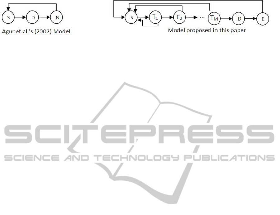
Figure 2: Comparison of Agur et al.'s (2002) model and the model proposed in this paper.
the set of all vertices such that their distances from v
do not exceed n. We write B(v, n) = {u ∈ V |ρ(u, v) ≤
n}. B(v, n) defines the near neighborhood of size n
of vertex v.
If U ⊆ V is a nonempty subset of vertices then
for every v ∈ V let ρ
U
(v) = min
u
∈
U
ρ(u, v) be the
minimum distance between v and another vertex u
contained in set U.
A state of a vertex is a 1-tuple, a 2-tuple or a 3-
tuple depending on the cell type. The first coordinate
denotes the cell’s type (S, T, D or E denoting a stem
cell, a transitive cell, a differentiated cell or an
empty space respectively). For a stem cell, the
second coordinate denotes the direction of
proliferation and the third coordinate denotes the
simulated time τ as an internal counter. For a
transition cell, the second coordinate denotes its
generation (progeny) while the third coordinate
denotes the simulated time. A differentiated cell has
only two coordinates and the second coordinate
denotes the simulated time. Finally, an empty space
does not have any counter or any other property,
thus it has a single coordinate that denotes the type.
Let µ be the maximum number of immediate
neighbors possible for any cell. µ also denotes the
number of directions for a stem cell to proliferate. A
stem cell, when it proliferates, can occupy an empty
space, if available, in its immediate neighborhood.
A transitive cell can go through several
generations (progeny) before it converts to a
differentiated cell. A transitive cell moves from one
generation to another after its internal counter
reaches a certain threshold. There are M generations
for a transitive cell, where M is greater than or equal
to 1. When a transitive cell has moved into its last
generation (i.e. M
th
generation) and when its internal
counter reaches a threshold, it converts to a
differentiated cell. In circumstances when there is
not even a single stem cell in the near neighborhood
of a transitive cell, a transitive cell converts back to
a stem cell. The rules given below also capture the
fact that a transitive cell’s ability to convert back to
a stem cell diminishes with each subsequent
generation. Let η denote the distance multiple for a
transitive cell to convert back to a stem cell. Thus,
the conversion from a transitive cell to a stem cell
depends on the distance multiple η and its current
generation.
Let Ω be the set of states of a vertex.
A map x: V → Ω is the state of the entire graph. The
set of all the states of the bone marrow graph G is
denoted by Ω
V
. A state x ∈ Ω
V
of the bone marrow
graph G at time t is denoted by x
t
. The state of a
vertex v at time t is denoted by x
t
(v).
With the above definitions, we are now ready to
define the rules of an iterative operator on all states
Ω
V
. It depends on three positive nonzero integers Φ,
Ψ, and Θ. The rules for the state changes can be
regarded as describing a family of cellular automata.
The first sub-rule of rule (1) states that a stem
cell converts to a transitive cell, if its internal
counter representing its cycling phase has reached a
threshold Ψ and its immediate neighborhood consists
only of stem cells. This corresponds to receiving a
signal that the microenvironment is saturated with
stem cells. The evidence for such a feedback is
provided by De Haan et al. (1996), where the
authors show that Hemopoietic cell amplification in
vivo is regulated by various mechanisms that appear
to be under control of many Hemopoietic growth
factors, including the activation and deactivation of
the quiescent stem cells into the cell cycle. The
second sub-rule within this rule specifies that if a
stem cell’s internal counter has reached a threshold
Ψ but its immediate neighborhood is not saturated by
stem cells, then the stem cell enters into a quiescent
state, i.e. it retains the same state. The third sub-rule
states that when a stem cell’s internal counter
reaches a threshold Ψ and there exists an empty
space in its neighborhood, then it proliferates such
that one of its descendants occupies the empty space
and the other remains in the original location. The
sub-rule also defines that the new stem cell as well
as the stem cell at original location receive the
renewed biological time. With this sub-rule, we also
denote a systematic way of choosing the empty
space for proliferation. The method we propose is by
adding a directional component d in the state of
every stem cell and by arranging all the possible
directions µ in a circular (round-robin) order. A stem
cell proliferates in the empty space in the direction
of the directional component d of its state. If the
direction given by the directional component d of
BIOINFORMATICS 2012 - International Conference on Bioinformatics Models, Methods and Algorithms
18
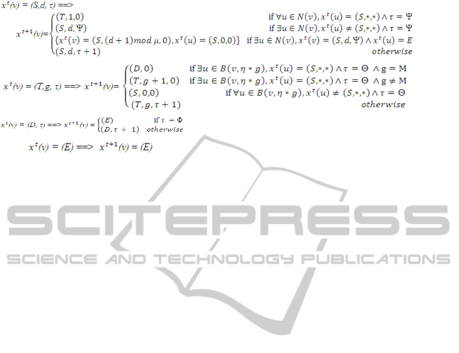
(1)
(2)
(3)
(4)
the state is occupied by any cell, then the stem cell
continues to choose the next direction, in the round-
robin order, for availability of the empty space.
After proliferation, the directional component of
stem cell is incremented to point to the next
direction. The last sub-rule states that if the internal
counter of a stem cell has not reached a threshold Ψ
then it is just incremented.
Transitive cells are intermediate cells that can
convert back to stem cells if there are not enough
stem cells in their near neighborhood, a situation that
can occur following radiation or organ damage.
Theise and Harris (2006) detail the dedifferentiation,
i.e., reversion of an intermediate cell into a stem cell.
Rule (2) states that when a transitive cell’s internal
counter reaches a threshold Θ it moves on to the
next generation unless it is not in its last (M
th
)
generation. If a transition cell’s counter has reached
the threshold Θ and it is in its last generation then it
gets converted to a differentiated cell. In certain
circumstances when a transitive cell does not have
any stem cell in its near neighborhood then it gets
converted back to a stem cell. The near
neighborhood is governed by a constant η and the
generation of the transitive cell. The stem cell like
property of a transitive cell goes on decreasing with
subsequent generations. The near neighborhood size
to find a stem cell keeps on increasing with each
subsequent generation of a transitive cell, implying
its reduced capacity to regenerate and the
requirement of an even stronger signal to convert
back to a stem cell.
Rule (3) states that when a differentiated cell’s
internal counter reaches a threshold time Φ, it
maturates. After maturation, the cell migrates to the
blood stream leaving the original space occupied by
the differentiated cell as empty space.
Rule (4) specifies that an empty space does not
change by itself. It does not have any internal
counter nor is involved in any computation.
We show next that the proposed model has
strong homeostatic properties, similar to Agur et
al.’s model.
3 HOMEOSTASIS PROPERTY OF
THE BONE MARROW MODEL
We begin by investigating the property of stem cells
to expand throughout the bone marrow. The
following lemma shows that any point in the bone
marrow graph gets occupied by a stem cell, given
that initially there is at least one stem cell in the
bone marrow graph.
Lemma 1. For any Φ, Ψ, Θ if there exist two vertices
u, v ∈ V such that at some time t, vertex v is not
occupied by a stem cell and u is, then there exists an
s > 0 such that v will be occupied by a stem cell at
time t + s.
Proof: From rule (1), we conclude that if u and v are
neighbors then u remains a stem cell as long as v is
not a stem cell. The vertex v itself turns into a stem
cell in no more than Φ+μΨ time steps. This is the
maximum time required including the time required
for cell at vertex v to migrate to the blood stream (in
case it was a differentiated cell), turn into an empty
space and as it is a neighbor of a stem cell, become a
stem cell after a maximum μΨ time steps. We can
use induction on the distance ρ(u, v) to obtain a
bound on the time that is needed for v to turn into a
stem cell:
s ≤ Φ + μ ρ(u, v)
Ψ (5)
The proof above conveys that the distance ρ
U(t)
(v)
between a vertex v, which is not occupied by a stem
cell at time t, to the subset U(t) ⊆ V of vertices
which includes a stem cell vertex at time t is a non-
increasing function. Furthermore, there exists s ≤ Φ
+ μρ
U(t)
(v)Ψ such that ρ
U(t+s)
(v) = 0.
We now show that if r ≥ t + s then ρ
U(r)
(v) ≤ Mη
in any two consecutive time slots. This means that
from the time t + s onwards there always is a stem
A DETERMINISTIC MODEL OF BONE MARROW WITH HOMEOSTATIC PROPERTIES AND WITH STEADY
PRODUCTION OF DIFFERENTIATED CELLS
19

cell not farther than Mη edges from v in any two
consecutive time slots.
Lemma 2. Suppose that a vertex v becomes a stem
cell at time t
0
, then for every t ≥ t
0
there is a vertex u
∈ B(v, Mη) which is occupied by a stem cell at time t
or t+1.
Proof: A necessary condition for the production of a
stem cell at a vertex v at time t
0
is that ∃v’ ∈ N(v),
x
t
0
−1
(v’) = (S,*, Ψ). Now, the cell at vertex v remains
a stem cell until last three conditions of rule (1) hold.
Therefore, if the cell at vertex v becomes a transitive
cell at time t
1
> t
0
, either it still has a stem cell
neighbor at time t
1
or all of its neighbors become
transitive cells simultaneously with v. If it is the first
scenario then we are done. The second scenario can
happen only if all the stem cells have their internal
counters synchronized and reach the threshold Ψ
simultaneously at time t
1
. In such a case, either there
is a stem cell in the near neighborhood of size Mη or
the vertex v will again convert from a transitive cell
to a stem cell at time t
1
+ 1 as all its near neighbors
are not stem cells. Thus if v is not a stem cell, there
is a stem cell in B(v, Mη) at time t
1
or t
1
+1. Applying
Lemma (1) ensures that until the next time the vertex
v is occupied by a stem cell, the distance from v to
the closest stem cell will not exceed Mη in any two
given consecutive time instances.
A direct conclusion from Lemma (2) is the
estimation for the density of stem cells in bounded
vicinity. We state the same in the following lemma
for graphs with bounded degree. The bone marrow
can be described as a graph of bounded degree with
each vertex connected only to its adjacent vertices.
We need two more notations:
If the graph G has the property that there exists Δ
such that |N(v)| ≤ Δ, ∀v ∈ V, we say that G has
bounded degree, and write deg(G) ≤ Δ.
The density of stem cells in a given finite subset of
vertices U ⊂ V at time t is the proportion at time t of
the number of stem cells S in U and the total number
of vertices in U. It is denoted by δ
t (U).
Lemma 3. Let G be a graph of bounded degree.
Suppose that at some time t
0
a vertex v is occupied
by a stem cell, then for every ball B = B(v, Mη) ⊂ G,
limt→∞ δt (B) ≥ 1/(2*(Δ
Mη
+ 1)).
Proof: By Lemma (1) and Lemma (2), any ball of
radius Mη admits a stem cell from a certain moment
on for any two consecutive time slots. The size of
such a ball contains less than or equal to Δ
Mη
+ 1
vertices.
In essence Lemma (1), Lemma (2) and Lemma (3)
show that not only is it true that one stem cell is
sufficient to bring back the bone marrow system
homeostasis, it is also true that the bone marrow has
a built-in mechanism guaranteeing that stem cells do
not become too scattered. Every ball of radius Mη is
occupied by at least one stem cell at any two
consecutive time steps from the moment it was
occupied by a first stem cell.
4 STEADY PRODUCTION OF
DIFFERENTIATED CELLS
We have seen that stem cells do fill the bone marrow
graph nicely. In this subsection, we show that the
system almost always generates enough mature
differentiated blood cells. Before proving the same,
we mention some observations:
• When a transitive cell is created and if it has a
stem cell neighbor, then it would always proceed to
create a differentiated cell. The stem cell neighbor
will remain a stem cell at least till the time a
transitive cell becomes a differentiated cell, the
differentiated cell becomes an empty space and the
empty space is occupied by another stem cell.
• Starting from non-saturated, if the complete
available space is to be saturated with stem cells
then every stem cell should divide into two stem
cells and any stem cell should not convert to a
transitive cell. If any stem cell converts to a
transitive cell, then the condition above will ensure
that it becomes a differentiated cell.
An extreme situation can occur, when the system
contains only stem cells at a time t and the internal
counters of all stem cells are synchronized. In such a
case, all the stem cells will convert to transitive cells
on or before t + Ψ. At the next time instant, all these
transitive cells will convert back to stem cells, as
there will not be a single stem cell in their near
neighborhood. This system would not produce any
differentiated cells, but will also not die out. We can
call such a state as resonant state as the cells will
resonate between stems cells and transitive cells
without producing any differentiated cells.
A resonant state can occur for a block of holding
capacity of 2
μ
cells if it is occupied completely by
stem cells starting from a single stem cell in μΨ
number of time steps. The physical occupancy of
stem cells in a given block depends largely on the
round-robin way of choosing the directions and
BIOINFORMATICS 2012 - International Conference on Bioinformatics Models, Methods and Algorithms
20

initial stem cell population. If the manner in which
the round-robin arrangement of directions is
clockwise or counter-clockwise then the resonant
state would not occur, if starting with a single cell in
two dimensional space as 2
μ
/μ
2
is greater than 1
when μ is greater than 4. For example, with μ = 8 in
a two dimensional space, 2
8
= 512 thus in 8Ψ time
steps 512 cells would be generated, but the ball of
radius 8 from the vertex v can hold only (8+1+8)
2
=
289 number of cells. Thus, some stem cell would be
surrounded by stem cells within 8Ψ time steps and it
would convert to a transitive cell. The possibility of
reaching a resonant state drops further after
considering the co-ordination of a similar event in
neighboring blocks.
A resonant state would occur if all the cell
positions are occupied by stem cells and their
internal time is also synchronized. This is an
extreme case. Thus, there are very few resonant
states out of the total number of states and hence,
there is a very low possibility that the model will be
in a resonant state.
Lemma 4. Suppose that a vertex v ∈ V is occupied by
a stem cell or a transitive cell at time t. Then either v
or one of its near neighbors in B(v, Mη) will be
occupied by a differentiated cell within (μ+1)Ψ +
(M+1)Θ + 1 iterations unless the system is in a
resonant state.
Proof: Assume that at vertex v there is a stem cell
that has no differentiated neighbors, otherwise we
are done. N(v) will consist only of stem cells by at
most μΨ time steps. Then v or one of its neighbors
will convert to a transitive cell after Ψ time steps.
Such a transitive cell will always have stem cells in
near neighborhood. Then after M generations of a
transitive cell, it would convert to a differentiated
cell, i.e. after (M+1)Θ time steps.
If v is a transitive cell and if v has a stem cell in its
near neighborhood then after (M+1)Θ time steps it
becomes a differentiated cell. If v is a transitive cell
and if v does not have any stem cell in its near
neighborhood, it becomes a stem cell in the next
time instance and the argument above follows.
Thus, except in the case of a resonant state, there
is a differentiated cell every (μ+1)Ψ + (M+1)Θ + 1
iterations in B(v, Mη).
Lemma (4) shows that in an eventuality of a
severe perturbation, a transitive cell will convert
back to a stem cell and bring back the entire system
to a steady state as shown in Lemma (3).
Note that in this model, one cannot guarantee
that a particular stem cell will eventually be
converted to a differentiated cell. The lemma above
does guarantee that in the close vicinity of any stem
cell some cell differentiates during a fixed bounded
time interval unless the system is not in a resonant
state. An immediate consequence of this is a lower
bound on the supply of differentiated cells to the
blood stream.
Corollary 5. Suppose that at some time t
0
a vertex v
is occupied by a stem cell, then every ball of radius
2Mη eventually supplies at least one mature cell
every (μ+1)Ψ + (M+1)Θ +1 + Φ time steps unless
the system is in a resonant state.
Proof: By Lemma (3), every ball of radius Mη
admits a stem cell from a certain moment onwards in
any two consecutive time instances. Lemma (4) says
that either this cell or one of its near neighbors (and
so we argue about balls of radius 2Mη) converts to a
differentiated cell within (μ+1)Ψ + (M+1)Θ +1 time
steps and migrate from the bone marrow as mature
cells after Φ additional time steps. Thus, every ball
of radius 2Mη eventually supplies at least one
mature cell every (μ+1)Ψ + (M+1)Θ + 1 + Φ time
steps.
5 STEADY STATES AND DYING
OUT STATES OF THE BONE
MARROW MODEL
We consider the unique state satisfying ∀v ∈ V, x(v)
= (E) ∨ x(v) = (D,*) as the death state of the system.
A state x
t
for which there exists a k ∈ Z
+
such that x
t+k
is the death state, will be called a dying out state.
Thus, a state not consisting of a single stem cell or a
transitive cell is a dying out state. We claim that
there is no other dying out state.
Lemma 6. The dying out states are only those
consisting of no stem cells or no transitive cells.
Proof: Let x
t
∈ Ω be a state, which is not one of the
dying out states. If there exists v ∈ V which is not a
stem cell at time t and since there exists a stem cell
at time t, v turns to a stem cell by Lemma (1). So by
Lemma (2) there is always a stem cell in B(v, Mη) in
any two consecutive time instants from the time v
has converted to a stem cell. The system does not die
out. Even if v is a transitive cell then it will become
a stem cell if there is no stem cell in its near
neighborhood.
Assume, therefore, that V admits only stem cells at
time t. If the counters are not synchronized they do
A DETERMINISTIC MODEL OF BONE MARROW WITH HOMEOSTATIC PROPERTIES AND WITH STEADY
PRODUCTION OF DIFFERENTIATED CELLS
21

not convert to transitive cells at the same time
instance and the system does not die out. If the
counters are synchronized they enter into resonant
state and again the system does not die out.
Thus, we have proved that the model
representing the bone marrow is dynamic in the
sense that it continuously changes in its constitution
and arrangement, and these changes occur at varying
rates depending on the constants Φ, Ψ, and Θ. We
have also seen that except for the death state, the
system never dies out. The bone marrow is in the
state of a dynamic equilibrium that can be
considered as if it is in homeostasis.
If there exist states x ∈ Ω in which for all k ∈ Z
+
,
x
t+k
= x
t
, then these are the steady states of the
system.
Lemma 7. For every Φ, Ψ, Θ the model does not
have steady states other than the death state and the
resonant state.
Proof: The fact that each differentiated cell matures
and leaves the bone marrow eventually, combined
with Lemma (1) and Lemma (6) implies the above.
6 DISCUSSION
In this paper, we have proposed a biologically
feasible model of bone marrow by extending the
model of Agur et al. (2002). The proposed model
adds the ability to recover from severe perturbations
of the bone marrow by adding rules that can convert
a transitive cell back to a stem cell and bring back
the system homeostasis.
The main properties of our model are achieved
from the feedback demand of rule (1), namely that a
stem cell does not convert to a transitive cell unless
its immediate microenvironment is saturated with
stem cells. The feedback demand in rule (2) is also
significant in the sense that a transitive cell can
convert back to a stem cell in cases of severe
perturbations resulting into loss of several stem
cells. We obtain the results that stem cells are
eventually dense (Lemma 2 and Lemma 3) and that,
let alone the case when there is no stem cell or
transitive cell, the system never dies out (Lemma 6).
Even though our extension of the Agur et al.’s
model is simple, the properties that emerge are
general, and hold for more complex descriptions. It
is a step ahead in the direction to model the
immensely complex bone marrow system.
Our extension of Agur et al.’s model removes all
the drawbacks associated with it. To summarize:
1. Our model has empty spaces but they no longer
need any counters.
2. In the model, a stem cell division is explicitly
represented.
3. The model has incorporated a directional
component for the division of stem cells.
4. A stem cell’s internal counter comes back to its
initial state after division; i.e. it becomes a true
daughter stem cell. Thus, a stem cell divides into
two identical daughter stem cells.
5. Transitive cells that have limited ability to
convert back to stem cells are represented in our
model. Their ability to regenerate to a stem cell
diminishes with subsequent generations.
6. One stem cell divides into a single empty space.
For another division, the stem cell has to wait for its
internal counter to reach a threshold as its internal
counter gets reset after division.
Our model overcomes all the drawbacks of Agur et
al.’s (2002) model. It also does not require message
passing between cells and the controlling
microenvironment, as required by the model of
d’Inverno and Saunders (2005). Hence, it is closer to
biological reality. The validation of this fact is
underscored by the agent-based simulations that we
have carried out. The results of these simulations are
included in the Appendix. These simulations also
demonstrate that, as predicted, large fractions of
stem cells do remain in the quiescent state (Gordon,
2007).
There are several other options of bringing the
model even more closer to biologically observed
complexity. There are two extensions that we would
like to work on in the future. The first is to make a
provision of apoptosis (cell death) for all types of
cells. Secondly, we can provide a stochastic
behavior for the stem cell proliferation to capture
variations in the human hematopoietic system.
Addition of the stochastic behavior will also enable
the introduction of a randomized directional
component. We would also like to increase the scale
of the simulation of the bone marrow system and to
perform the same in three-dimensional space,
typically with simulated bone marrow size that can
hold 10
8
to 10
12
number of cells and with the model
constants matching observed parameters (Michor,
Hughes, Iwasa, Branford, Shah, Sawyers and
Nowak, 2005).
REFERENCES
Agur Z., Daniel Y. and Ginosar Y. (2002). The Universal
BIOINFORMATICS 2012 - International Conference on Bioinformatics Models, Methods and Algorithms
22
Properties of Stem Cells as pinpointed by a Simple
Discrete Model. In Journal of Mathematical Biology,
44(1):79-86.
De Haan G., Dontje B. and Nijhof W. (1996). Concepts of
Hemopoietic Cell Amplification. Synergy,
Redundancy, and Pleiotropy of Cytokines affecting the
Regulation of Erythropoiesis. In Leukemia Lymphoma,
22(5-6):385-94.
Gordon M. (2007). Stem Cells and Haemopoiesis. In
Hoffbrand A., Catovsky D. and Tuddenhan E. (Eds.),
Postgraduate Haematology, pp. 1-12. Blackwell
Oxford, 5
th
edition.
d’Inverno M. and Saunders R. (2005). Agent-based
Modeling of Stem Cell self-organization in a Niche,
Engineering Self- Organizing Systems: Methodologies
and Applications. In Brueckner S., Di Marzo G.,
Serugendo, Karageorgos A. and Nagpal R. (Eds.),
LNAI, 3464. Springer.
Michor F., Hughes T., Iwasa Y., Branford S., Shah N.,
Sawyers C. and Nowak M. (2005). Dynamics of
chronic myeloid leukaemia. In Nature
435(7046):1267-70.
O'Neill A. and Schaffer D. (2004). The biology and
engineering of stem-cell control. In Biotechnology and
Applied Biochemistry 40(Pt 1):5-16.
Roeder I. and Radtke F. (2009). Stem Cell Biology meets
Systems Biology. In Development 136(21):3525-30.
Theise N. and Harris R. (2006). Postmodern Biology:
(Adult) (Stem) Cells Are Plastic, Stochastic, Complex,
and Uncertain. In Handbook of Experimental
Pharmacology (174): 389-408.
APPENDIX
An agent-based model was developed for the bone
marrow system proposed in this paper. We have
implemented the program in the C programming
language and it is available at the following website:
http://sites.google.com/site/stemcellmodel.
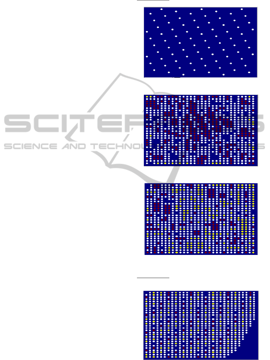
The results given below are on a two
dimensional grid of size 30 x 30 for the following
constants:
Φ = 4 Constant for differentiated cells.
Ψ = 1 Constant for stem cells.
Θ = 1 Constant for transitive cells.
η = 2 Constant for distance measure for near
neighborhood from a particular transitive cell.
μ = 8 Number of directions in a 2-D space.
M = 3 Number of generations of transition cells.
We specified colors like Silver (S), Titanium Yellow
(T), and Dark Red (D) to stem cells, transitive cells,
and differentiated cells respectively. Also note that
the directional component moves in the clockwise
manner.
Simulation 1:
Starting with 10% stem cells
Figure 3: Initial Screen (with 10% stem cells).
Figure 4: After 100 time steps, 93.3% stem cells quiescent.
Figure 5: After 3000 time steps, 88% stem cells quiescent.
Simulation 2: Starting with single stem cell at top
left.
Figure 6: After 100 time steps, 91.9% stem cells quiescent.
A DETERMINISTIC MODEL OF BONE MARROW WITH HOMEOSTATIC PROPERTIES AND WITH STEADY
PRODUCTION OF DIFFERENTIATED CELLS
23
