CHARACTERIZING RELATIONSHIPS THROUGH

CO-CLUSTERING

A Probabilistic Approach

Nicola Barbieri, Gianni Costa, Giuseppe Manco and Ettore Ritacco

High Performance Computing and Networking Institute of the Italian National Research Council

v. Pietro Bucci 41C, Arcavacata di Rende (CS), Italy

Keywords:

Collaborative ﬁltering, Recommender systems, Block clustering, Co-clustering.

Abstract:

In this paper we propose a probabilistic co-clustering approach for pattern discovery in collaborative ﬁltering

data. We extend the Block Mixture Model in order to learn about the structures and relationships within pref-

erence data. The resulting model can simultaneously cluster users into communities and items into categories.

Besides its predictive capabilities, the model enables the discovery of signiﬁcant knowledge patterns, such as

the analysis of common trends and relationships between items and users within communities/categories. We

reformulate the mathematical model and implement a parameter estimation technique. Next, we show how

the model parameters enable pattern discovery tasks, namely: (i) to infer topics for each items category and

characteristic items for each user community; (ii) to model community interests and transitions among topics.

Experiments on MovieLens data provide evidence about the effectiveness of the proposed approach.

1 INTRODUCTION

Collaborative Filtering (CF) is recently becoming the

dominant approach in Recommender Systems (RS).

In literature, several CF recommendation techniques

have been proposed, mainly focusing on the predic-

tive skills of the system. Recent studies (McNee et al.,

2006; Cremonesi et al., 2010) have shown that the fo-

cus on prediction does not necessarily helps in devis-

ing good recommender systems. Under this perspec-

tive, CF models should be considered in a broader

sense, for their capability to understand deeper and

hidden relationships among users and products they

like. Examples in this respect are user communi-

ties, item categories preference patterns within such

groups. Besides their contribution to the minimiza-

tion of the prediction error, these relationships are im-

portant as they can provide a faithful yet compact de-

scription of the data which can be exploited for better

decision making.

In this paper we present a co-clustering approach

to preference prediction and rating discovery, based

on the Block Mixture Model (BMM) proposed in (Go-

vaert and Nadif, 2005). Unlike traditional CF ap-

proaches, which try to discover similarities between

users or items using clustering techniques or ma-

trix decomposition methods, the aim of the BMM

is to partition data into homogeneous block enforc-

ing a simultaneous clustering which consider both

the dimension of the preference data. This approach

highlights the mutual relationship between users and

items: similar users are detected by taking into ac-

count their ratings on similar items, which in turn are

identiﬁed considering the ratings assigned by similar

users. We extended the original BMM formulation

to model each preference observation as the output

of a gaussian mixture employing a maximum likeli-

hood (ML) approach to estimate the parameter of the

model. Unfortunately, the strict interdependency be-

tween user and item cluster makes difﬁcult the appli-

cation of traditional optimization approaches like EM.

Thus, we perform approximated inference based on a

variational approach and a two-step application of the

EM algorithm which can be thought as a good com-

promise between the semantic of the original model

and the computational complexity of the learning al-

gorithm.

We reformulate standard pattern discovery tasks

by showing how a probabilistic block model automat-

ically allows to infer patterns and trends within each

block. We show experimentally that the proposed

model guarantees a competitive prediction accuracy

with regards to standard state-of-the art approaches,

and yet it allows to infer topics for each item cate-

Barbieri N., Costa G., Manco G. and Ritacco E..

CHARACTERIZING RELATIONSHIPS THROUGH CO-CLUSTERING - A Probabilistic Approach.

DOI: 10.5220/0003656800640073

In Proceedings of the International Conference on Knowledge Discovery and Information Retrieval (KDIR-2011), pages 64-73

ISBN: 978-989-8425-79-9

 2011 SCITEPRESS (Science and Technology Publications, Lda.)

gory, as well as to learn characteristic items for each

user community, or to model community interests and

transitions among topics of interests. Experiments on

both the Netﬂix and Movielens data show the effec-

tiveness of the proposed model.

2 PRELIMINARIES AND

RELATED WORK

User’s preferences can be represented by using a

M × N rating matrix R, where M is the cardinality of

the user-set U = {u

,··· ,u

} and N is the cardinal-

ity of the item-set I = {i

,··· ,i

}. The rating value

associated to the pair hu,ii will be denoted as r

. Typi-

cally the number of users and items can be very large,

with M >> N, and preferences values fall within a

ﬁxed integer range V = {1,··· ,V}, where 1 denote

the lower interest value. Users tend to express their

interest only on a restricted number of items; thus,

the rating matrix is characterized by an exceptional

sparseness factor (e.g more than 95%). Let δ(u,i) be

a rating-indicator function, which is equals to 1 if the

user u has rated/purchased the item i, zero otherwise.

Let I (u) denote the set of products rated by the user

u: I(u) = {i ∈ I : δ(u, i) = 1}; symmetrically, U(i)

denotes the set of users who have expressed their pref-

erence on the item i.

Latent Factor models are the most representative

and effective model-based approaches for CF. The un-

derlying assumption is that preference value associ-

ated to the pair hu,ii can be decomposed considering

a set of contributes which represent the interaction be-

tween the user and the target item on a set of features.

Assuming that there are a set of K features which de-

termine the user’s interest on an given item. The as-

sumption is that a rating is the result of the inﬂuence

of these feature to users and items: ˆr

∑

z=1

u,z

z,i

where U

u,z

is the response of the user u to the feature

z and V

z,i

is the response on the same feature of the

item i.

Several learning schema have been proposed to

overcome the sparsity of the original rating matrix

and to produce accurate models. The learning phase

may be implemented in a deterministic way, via gra-

dient descent (Funk, 2006) or, following a proba-

bilistic approach, maximizing the log-likelihood of

the model via the Expectation Maximization algo-

rithm. The latter leads to the deﬁnition of the As-

pect Model(Hofmann and Puzicha, 1999), known

also as pLSA. According to the user community vari-

ant, the rating value r is conditionally independent

of the user’s identity given her respective commu-

nity Z; thus, the probability of observing the rat-

ing value r for the pair hu,ii can be computed as

p(r|u, i) =

∑

z=1

p(r|i, z)p(z|u), where P(z|u) mea-

sures how much the preference values given by u ﬁts

with the behavior of the community z and p(r|i,z) is

the probability that a user belonging to the community

z assigns a rating value r on i.

Only a few co-clustering approaches have been

proposed for CF data. An application of the weighted

Bregman coclustering (Scalable CC) to rating data is

discussed in (George and Merugu, 2005). The two-

sided clustering model for CF (Hofmann and Puzicha,

1999) is based on the strong assumption that each

person belongs to exactly one user-community and

each item belong to one groups of items, and ﬁ-

nally the rating value is independent of the user and

item identities given their respective cluster member-

ships. Let C =

{

,··· ,c

}

be the user-clusters and

let c(u) : U → C be a function that maps each user to

the respective cluster. Similarly, let D =

{

,··· ,d

}

be a set of disjoint item-clusters, and d(i) : I → D

is the corresponding mapping function. According to

the two-sided clustering model, the probability of ob-

serving the preference value r conditioned to the pair

hu,ii is the following:

p(r|u, i, c(u) = c, d(i) = d) = p(r|c, d)

where p(r|c, d) are Bernoulli parameters and the clus-

ter membership are estimated by employing a varia-

tional inference approach.

The Flexible Mixture Model (FMM) (Jin et al.,

2006) extends the Aspect and the two sided model, by

allowing each user/item to belong to multiple clusters,

which are determined simultaneously, according to a

coclustering approach. Assuming the existence of K

user clusters indexed by c and L item clusters, indexed

by d, and let p(c

) be the probability of observing

the user-cluster k with p(u|c

) being the probability

of observing the user proﬁle u given the cluster k and

using the same notations for the item-cluster, the joint

probability p(u,i,r) is deﬁned as:

p(u,i,r) =

∑

c=1

∑

d=1

p(c)p(d)p(u|c)p(i|d)p(r|c,d)

The predicted rating associated to the pair hu,ii is then

computed as:

ˆr

∑

r=1

p(u,i,r)

∑

p(u,i,r

)

The major drawback of the FMM relies on the com-

plexity of the training procedure, which is connected

with the computation of the probabilities p(c,d|u,i,r)

during the Expectation step.

A coclustering extension of the LDA(Blei et al., 2003)

CHARACTERIZING RELATIONSHIPS THROUGH CO-CLUSTERING - A Probabilistic Approach

model for rating data have been proposed in (Porte-

ous et al., 2008): the Bi-LDA employs two interacting

LDA models which enforce the simultaneous cluster-

ing of users and items in homogeneous groups.

Other co-clustering approaches have been pro-

posed in the current literature (see (Shan and Baner-

jee, 2008; Wang et al., 2009) ), however their exten-

sion to explicit preference data, which requires a dis-

tribution over rating values, has not been provided yet.

3 A BLOCK MIXTURE MODEL

FOR PREFERENCE DATA

In this section, we are interested in:devising how

the available data ﬁts into ad-hoc communities and

groups, where groups can involve both users and

items. Fig. Fig. 1 shows a toy example of prefer-

ence data co-clustered into blocks. As we can see,

a coclustering induces a natural ordering among rows

and columns, and it deﬁnes blocks in the rating matrix

with similar ratings. The discovery of such a structure

is likely to induce information about the population,

as well as to improve the personalized recommenda-

tions.

Formally, a block mixture model (BMM) can be

deﬁned by two partitions (z, w) which, in the case of

preference data and considering known their respec-

tive dimensions, have the following characterizations:

• z = z

,··· ,z

is a partition of the user set U into

K clusters and z

= 1 if u belongs to the cluster

k, zero otherwise;

• w = w

,··· ,w

is a partition of the item set I into

L clusters and w

= 1 if the item i belongs to the

cluster l, zero otherwise.

Given a rating matrix R, the goal is to determine such

partitions and the respective partition functions which

specify, for all pairs hu, ii the probabilistic degrees of

membership wrt. to each user and item cluster, in

such a way to maximize the likelihood of the model

given the observed data. According to the approach

described (Govaert and Nadif, 2005; Gerard and Mo-

hamed, 2003), and assuming that the rating value r

observed for the pair hu,ii is independent from the

user and item identities, ﬁxed z and w, the generative

model can be described as follows:

1. For each u generate z

∼ Discrete(π

;...;π

)

2. for each i generate w

∼ Discrete(ψ

;...;ψ

)

3. for each pair (u, i):

• detect k and l such that z

= 1 and w

= 1

• generate r ∼ N(µ

;σ

)

There are two main differences with respect to the

FMM model introduced in the related work. First

of all, in our model all cluster membership are as-

sumed given a-priori, whereas FMM models each

pair separately. That is, we assume that the clus-

ter memberships z

and w

are sampled once and for

all, whereas in the FMM model they are sampled for

each given pair (u, i). Thus, in the FMM model, a

use u can be associated to different clusters in differ-

ent situations. Although more expressive, this model

is prone to overﬁtting and makes the learning pro-

cess extremely slow. The second difference is in the

way we model the rating probability p(r|z,w). FMM

adopts the multinomial model, whereas we choose to

adopt the gaussian. The latter better weights the dif-

ference between the expected and the observed value:

i.e. larger values for |ˆr

− r

| introduce a penalty fac-

tor.

The corresponding data likelihood in the Block

Mixture can be modeled as

p(R,z,w) =

∏

u∈U

p(z

)

∏

i∈I

p(w

)

∏

(u,i,r)∈R

p(r|z

)

and consequently, the log-likelihood becomes:

(Θ;R,z,w) =

∑

k=1

∑

u∈U

logπ

∑

l=1

∑

i∈I

logψ

∑

hu,i,ri∈R

∑

logϕ(r; µ

,σ

)

where Θ represents the whole set of parameters

,...,π

, ψ

,...,ψ

, µ

,...,µ

, σ

,...,σ

and

ϕ(r; µ, σ) is the gaussian density function on the rat-

ing value r with parameters µ and σ, i.e., ϕ(r; µ; σ) =

(2π)

−1/2

−1

exp



−1

2σ

(r − µ)



In the following we show how the model can be

inferred and exploited both for prediction and for pat-

tern discovery.

3.1 Inference and Parameter

Estimation

Denoting p(z

= 1|u, Θ

(t)

) = c

, p(w

= 1|i, Θ

(t)

) =

and p(z

= 1|u,i,Θ

(t)

) = e

ukil

, The conditional

expectation of the complete data log-likelihood be-

comes:

Q(Θ;Θ

(t)

) =

∑

k=1

∑

logπ

∑

l=1

∑

logψ

∑

hu,i,ri∈R

∑

ukil

logϕ(r; µ

,σ

)

KDIR 2011 - International Conference on Knowledge Discovery and Information Retrieval

Figure 1: Example Co-Clustering for Preference Data.

As pointed out in (Gerard and Mohamed, 2003), the

above function is not tractable analytically, due to

the difﬁculties in determining e

ukil

; nor the adoption

of its variational approximation (e

ukil

= c

· d

) al-

lows us to derive an Expectation-Maximization pro-

cedure for Q

(Θ,Θ

(t)

) where the M-step can be com-

puted in closed form. In (Gerard and Mohamed,

2003) the authors propose an optimization of the

complete-data log-likelihood based on the CEM al-

gorithm. We adapt the whole approach here. First

of all, we consider that the joint probability of a a

normal population x

with i = 1 to n can be factored

as:

∏

i=1

ϕ(x

;µ,σ) = h(x

,...,x

)∗ ϕ(u

;µ,σ),

where h(x

,...,x

) = (2π)

−n/2

, ϕ(u

;µ,σ) =

−u

exp



µ−u

−u

2σ



and u

, u

and u

are the suf-

ﬁcient statistics.

Based on the above observation, we can deﬁne a

two-way EM approximation based on the following

decompositions of Q

(Θ,Θ

(t)

) = Q

(Θ,Θ

(t)

|d) +

∑

i∈I

∑

l=1

logψ

−

∑

u∈U

∑

i∈I (u)

/2log(2π)

where

(Θ,Θ

(t)

|d) =

∑

u=1

∑

k=1

(log(π

) + τ

)

∑

l=1

log



ϕ(u

(u,l)

;µ

,σ

)



(u,l)

∑

i∈I (u)

; u

(u.l)

∑

i∈I (u)

(u,l)

∑

i∈I (u)

)

Analogously,

(Θ,Θ

(t)

) = Q

(Θ,Θ

(t)

|c) +

∑

u∈U

∑

k=1

logπ

−

∑

i∈I

∑

u∈U(i)

/2log(2π)

where

(Θ,Θ

(t)

|c) =

∑

i=1

∑

l=1

(log(ψ

) + τ

)

∑

k=1

log



ϕ(u

(i,k)

(i.k)

(i,k)

;µ

,σ

)



(i,k)

∑

u∈I (u)

; u

(i,k)

∑

u∈I (u)

(i,k)

∑

u∈I (u)

)

The advantage in the above formalization is that

we can approach the single components separately

and, moreover, for each component it is easier to esti-

mate the parameters. In particular, we can obtain the

following:

1. E-Step (User Clusters):

= p(z

= 1|u) =

p(u|z

) · π

∑

p(u|z

) · π

p(u|z

) =

∏

l=1

ϕ(u

(u,l)

(u.l)

(u,l)

;µ

,σ

)

2. M-Step (User Clusters):

∑

u∈U

∑

u=1

∑

i∈I (u)

∑

u=1

∑

i∈I (u)

(σ

)

∑

u=1

∑

i∈I (u)

− µ

)

∑

u=1

∑

i∈I (u)

CHARACTERIZING RELATIONSHIPS THROUGH CO-CLUSTERING - A Probabilistic Approach

3. E-Step (Item Clusters):

= p(w

= 1|i) =

p(i|w

) · ψ

∑

p(i|w

) · ψ

p(i|w

) =

∏

k=1

ϕ(u

(i,k)

;µ

,σ

)

4. M-Step (Item Clusters):

∑

i∈I

∑

i=1

∑

u∈U(i)

∑

i=1

∑

u∈U(i)

(σ

)

∑

i=1

∑

u∈U(i)

− µ

)

∑

i=1

∑

u∈U(i)

3.2 Rating Prediction

The blocks resulting from a co-clustering can be di-

rectly used for prediction. Given a pair hu,ii, the

probability of observing a rating value r associated

to the pair hu, ii can be computed according to one of

the following schemes:

• Hard-Clustering Prediction:

p(r|i, u) = ϕ(r;µ

,σ

), where k =

argmax

j=1,··· ,K

u j

and l = argmax

h=1,···,L

are the clusters that better represent the ob-

served ratings for the considered user and item

respectively.

• Soft-Clustering Prediction:

p(r|i, u) =

∑

k=1

∑

l=1

ϕ(r; µ

,σ

), which

consists of a weighted mixture over user and item

clusters.

The ﬁnal rating prediction can be computed by using

the expected value of p(r|u, i).

In order to test the predictive accuracy of the

BMM we performed a suite of tests on a sample of

Netﬂix data. The training set contains 5, 714, 427 rat-

ings, given by 435, 656 users on a set of 2, 961 items

(movies). Ratings on those items are within a range

1 to 5 (max preference value) and the sample is 99%

sparse. The test set contains 3, 773, 781 ratings given

by a subset of the users (389, 305) in the training set

over the same set of items. Over 60% of the users

have less than 10 ratings and the average number of

evaluations given by users is 13.

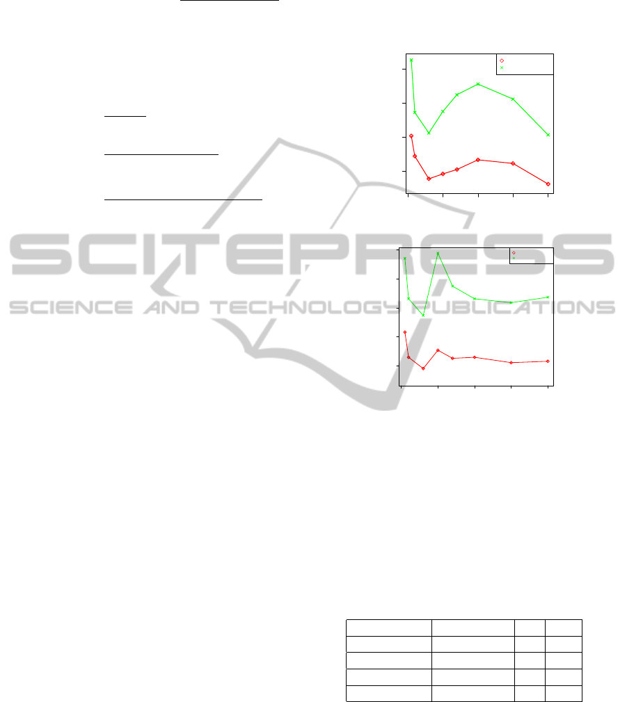
We evaluated the performance achieved by the

BMM considering both the Hard and the Soft predic-

tion rules and performed a suite of experiments vary-

ing the number of user and item clusters. Experiments

on the three models have been performed by retaining

the 10% of the training (user,item,rating) triplets as

held-out data and 10 attempts have been executed to

determine the best initial conﬁgurations. Performance

results measured using the RMSE for two BMM with

30 and 50 user clusters are showed in Fig. 2(a) and

Fig. 2(b), respectively. In both cases the soft cluster-

0 50 100 150 200

0.95 0.96 0.97 0.98

#Item Clusters

RMSE

Soft Clustering

Hard CLustering

(a) 30 user clusters

0 50 100 150 200

0.95 0.96 0.97 0.98 0.99

#Item Clusters

RMSE

Soft Clustering

Hard CLustering

(b) 50 userclusters

Figure 2: Predictive Accuracy of BMM.

ing prediction rule overcomes the hard one, and they

show almost the same trend. The best result (0.9462)

is achieved by employing 30 user clusters and 200

item clusters. We can notice from Tab. 1 that the re-

sults follow the same trend as other probabilistic mod-

els, like pLSA, which on the same portion of the data

achieves 0.9474 accuracy.

Table 1: RMSE of principal (co-)clustering approaches.

Method Best RMSE K H

BMM 0.946 30 200

PLSA 0.947 30 -

FMM 0.954 10 70

Scalable CC 1.008 10 10

4 PATTERN DISCOVERY USING

BMM

The probabilistic formulation of the BMM provides a

powerful framework for discovering hidden relation-

KDIR 2011 - International Conference on Knowledge Discovery and Information Retrieval

ships between users and items. As exposed above,

such relationships can have several uses in users seg-

mentation, product catalog analysis, etc. Several

works have focused on the application of clustering

techniques to discover patterns in data by analyzing

user communities or item categories. In (Jin et al.,

2004) authors showed how the pLSA model in its co-

occurrence version can be used to infer the underlying

task of a web browsing session and to discover rela-

tionships between users and web pages. Those ap-

proaches can be further reﬁned by considering the co-

clustering structure proposed so far, which increases

the ﬂexibility in modeling both user communities and

item categories patterns. Given two different user

clusters which group users who have showed a similar

preference behavior, the BMM allows the identiﬁca-

tion of common rated items and categories for which

the preference values are different. For example, two

user community might agree on action movies while

completely disagree on one other. The identiﬁcation

of the topics of interest and their sequential patterns

for each user community lead to an improvement of

the quality of the recommendation list and provide the

user with a more personalized view of the system. In

the following we will discuss examples of pattern dis-

covery and user/item proﬁling tasks.

The experiments in this section were performed

considering the 1M MovieLens dataset

, which con-

tains 1,000, 209 ratings given by 6, 040 users on ap-

proximately 3, 900 movies. Each user in this dataset

has at least 20 ratings and a list of genres is given for

each movie.The latter information will be used to val-

idate the the discovered block structure.

4.1 Co-clustering Analysis

The relationships between groups of users and items

captured by the BMM can be easily recognized by

analyzing the distribution of the preference values

for each cocluster. Given a co-cluster hk,li, we can

analyze the corresponding distribution of rating val-

ues to infer the preference/interest of the users be-

longing to the community k on item of the category

l. Fig. 3 shows graphically a block mixture model

with 10 users clusters and 9 item clusters built on

the MovieLens dataset. A hard clustering assign-

ment has been performed both on users and clus-

ters: each user u has been assigned to the cluster

c such that c = argmax

k=1,···,K

. Symmetrically,

each item i has been assigned to the cluster d such

that: d = argmax

l=1,···,L

. The background color

of each block hk,li describes both the density of rat-

http://www.grouplens.org/system/ﬁles/ml-data-

10M100K.tar.gz

Figure 3: Coclustering.

Table 2: Gaussian Means for each block.

3.4 3.59 3.59 4 2.91 4.43 3.59 2.93 3.65

2.23 2.2 2.92 2.79 2 3.45 2.07 1.80 2.51

2.11 3.24 3 3.66 2 4.17 1 1.03 5

2.45 2.69 2.54 3.2 2.43 3.74 2.51 2 2.56

1 1.79 1 2.32 1 2.98 1.66 1 1.75

2.93 3.07 3 3.57 2.20 4.09 2.9 2.3 3.16

1 3.56 3.9 3.7 3.64 3.39 4 3.49 2

2.25 2.26 1.62 3.27 1 4.17 4.54 1 2.45

4.08 3.24 4.40 3.54 5 4 3.71 4.5 5

1.91 2.82 1 2.7 4.3 2.2 1 4 2

ings and the average preference values given by the

users (rows) belonging to the k-th group on items

(columns) of the l-th category: the background inten-

sity increases with the average rating values of the co-

clusters, which are given in Tab. 2. Each point within

the coclusters represents a rating, and again an higher

rating value corresponds to a more intense color. The

analysis underlines interesting tendencies: for exam-

ple, users belonging to the user community c

tend

to assign higher rating values than the average, while

items belonging to item category d

are the most ap-

preciated. A zoom of portions of the block image is

given in Fig. 4(a) and in Fig. 4(b). Here, two blocks

are characterized by opposite preference behaviors:

the ﬁrst block contains few (low) ratings, whereas the

second block exhibit a higher density of high value

ratings.

4.2 Item-topic Analysis

A structural property of interest is the item-topic de-

CHARACTERIZING RELATIONSHIPS THROUGH CO-CLUSTERING - A Probabilistic Approach

(a) Cocluster (c

): Avg rating: 1

(b) Cocluster (d

): Avg rating: 4.43

Figure 4: Cocluster Analysis.

pendency. Given a set of F topics G =

{

,···g

}

and assuming that each item is tagged with at least

one of those, we can estimate the relevance of each

topic within item clusters through a variant of the tf-

idf measure (Wu et al., 2008), namely topic frequency

- inverse category frequency (tf-icf ).

The topic frequency (similar to the term fre-

quency) of a topic g in a cluster d

can be deﬁned as:

g,d

∑

i∈d

δ(g∈Q

)

∑

u∈U

δ(u,i)

∑

i∈d

δ(g

∈Q

)

∑

u∈U

δ(u,i)

In a scenario, where items are associated with sev-

eral topics (genres), and where the number of topics

is much lower than size of the itemset, it is high likely

that all topics appear at least one in each item cate-

gory. According to this consideration, the standard

deﬁnition of idf would be useless for our purposes.

We, hence, provide an alternative formulation based

on entropy (Shannon, 1951), namely inverse category

frequency (icf ) for a topic g is:

ic f

= 1+ p(g) log

[p(g)]+[1− p(g)] log

[(1− p(g))]

Here, p(g) represent the prior probability of ob-

serving a item-genre and is computed as p(g) =

∑

l=1

p(g|d

) · p(d

), where p(g|d

) = t f

g,d

and

p(d

) = ψ

By combining the above deﬁnitions we can ﬁnally

obtain the tf-icf measure for a topic g in a category d

as:

tf-icf

g,d

= tf

g,d

× icf

We can also exploit the fact that BMM provides a soft

assignment to clusters, and provide an alternative ver-

sion of tf as:

g,d

∑

i∈d

δ(g∈Q

)

· d

∑

u∈U

δ(u,i)

∑

i∈d

δ(g

∈Q

)

· d

∑

u∈U

δ(u,i)

The above considerations can be also applied to the

case of item frequency:

i,d

∑

u∈U

δ(u,i)

∑

∈d

∑

u∈U

δ(u,i

)

ic f

= 1 + p(i) log

[p(i)]

+[1 − p(i)]log

[(1 − p(i))]

where:

p(i) =

|U(i)|

|U|

The topic and item relevance described so far can

be directly employed to identify and measure the in-

terest of each user community into topics and items.

More speciﬁcally, we can measure the interest of a

user community c

for a topic g as:

,g) =

∑

l=1

· tf-icf

g,d

∑

l=1

· tf-icf

The item-based counterpart follows straightfor-

wardly:

,j) =

∑

l=1

· if-icf

j,d

∑

l=1

· if-icf

where j is the item target.

4.2.1 Evaluation

The MovieLens dataset provides for each movie a list

of genres. This information can be used to charac-

terize each item category, by exploiting the within-

cluster topic relevance discussed so far. The tf-icf

measure of observing each genre within each item

category is given in Tab. 3, where the dominant topic

is in bold.

The pie charts in Fig. 5(a), Fig. 5(b) and Fig. 5(c)

show the distribution on topics for different item clus-

ters. We can observe different patterns: d

is char-

acterized by a strong attitude for horror movies, an-

imation is the dominant topic in cluster 6, and d

summarized by the war genre. Finally, the cluster d

shows a predominance of drama movies. A summary

of the dominant genres in each item cluster, i.e., with

higher tf-icf, is given below:

Item Cluster Dominant Genre

Drama

Horror

Action

Drama

Animation

Comedy

War

Documentary

Fig. 6 shows the CI

(g,c

) values (in gray scale).

We can further analyze such values to infer the inter-

KDIR 2011 - International Conference on Knowledge Discovery and Information Retrieval

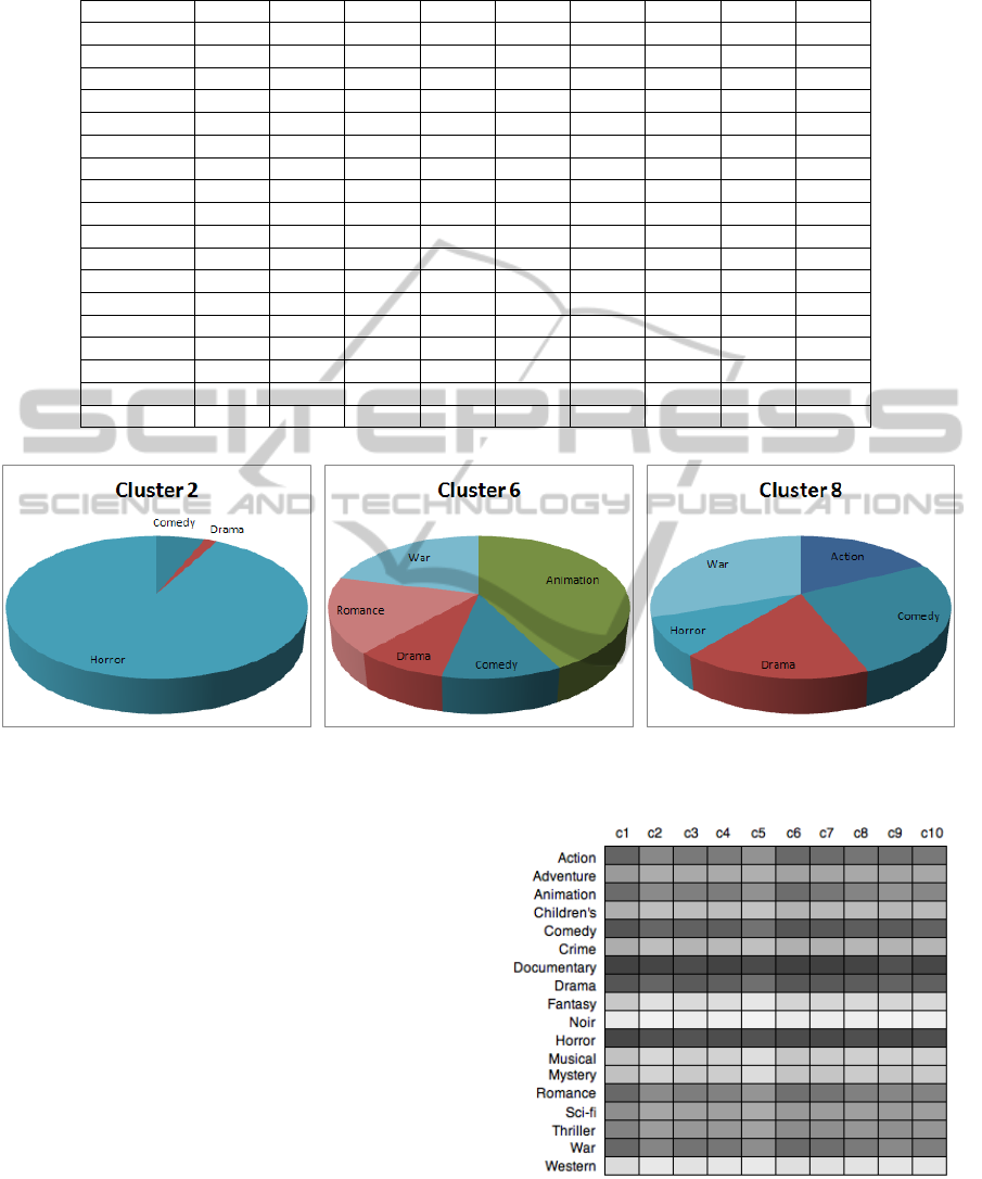
Table 3: tf-icf measures for each genre in each movie category

Action 0.03640 0 0.07375 0.06054 0.05152 0 0.05624 0.06966 0

Adventure 0.01981 0 0.04237 0.04339 0.03813 0 0.03828 0 0

Animation 0.01591 0 0.00660 0.00926 0.01801 0.24622 0.00999 0 0

Children’s 0.01581 0 0.03228 0.01643 0.02261 0 0.02855 0 0

Comedy 0.04137 0.03559 0.05403 0.05185 0.04730 0.06209 0.05685 0.10228 0

Crime 0.03319 0 0.01585 0.02217 0.01973 0 0.02515 0 0

Documentary 0.01423 0 0.00028 0.00053 0.00291 0 0.00341 0 0.94466

Drama 0.09777 0.00923 0.02308 0.05247 0.07720 0.04839 0.05099 0.06727 0

Fantasy 0.00553 0 0.01175 0.01579 0.01171 0 0.01559 0 0

Film-Noir 0.01485 0 0.00029 0.00123 0.00580 0 0.00113 0 0

Horror 0.01570 0.53057 0.08225 0.02691 0.01569 0 0.04014 0.03426 0

Musical 0.01739 0 0.00619 0.00914 0.02224 0 0.01088 0 0

Mystery 0.01697 0 0.00832 0.02757 0.00958 0 0.00952 0 0

Romance 0.03470 0 0.02395 0.05776 0.05092 0.09889 0.04625 0 0

Sci-Fi 0.02818 0 0.06247 0.04644 0.03843 0 0.04150 0 0

Thriller 0.04613 0 0.05851 0.05052 0.04771 0 0.05057 0 0

War 0.03902 0 0.01268 0.01041 0.01442 0.12291 0.00716 0.11860 0

Western 0.01653 0 0.00625 0.00704 0.00641 0 0.00875 0 0

(a) Item cluster 2 (b) Item cluster 6 (c) Item cluster 8

Figure 5: Topic Analysis on Item Clusters.

est of a user community for a given topic. In particu-

lar, a community exhibits a high interest for a topic if

the corresponding CI

value is sufﬁciently higher than

the average CI

value of all the other topics. Table

4 summarizes the associations among user communi-

ties and item topics. For example, users in c

exhibit

preferences for the Action and War genres.

4.3 User Proﬁle Segmentation

The topics of interest of a user may change within

time and consecutive choices can inﬂuence each

other. We can analyze such temporal dependencies by

mapping each user’s choice into their respective item

cluster. Assume that movieLens data can be arranged

as a set { ¯u

,..., ¯u

}, where ¯u =

{

,i,t

i∀i ∈ I (u)

}

and t

is the timestamp corresponding to the rating

given by the user u on the item i. By chronologically

sorting ¯u and segmenting it according to item clus-

ter membership, we can obtain a view of how user’s

Figure 6: Topic-Interests for User Communities.

tastes change over time. Three example of user pro-

ﬁle segmentation are given in the ﬁgures below (the

mapping between item categories and colors is given

CHARACTERIZING RELATIONSHIPS THROUGH CO-CLUSTERING - A Probabilistic Approach

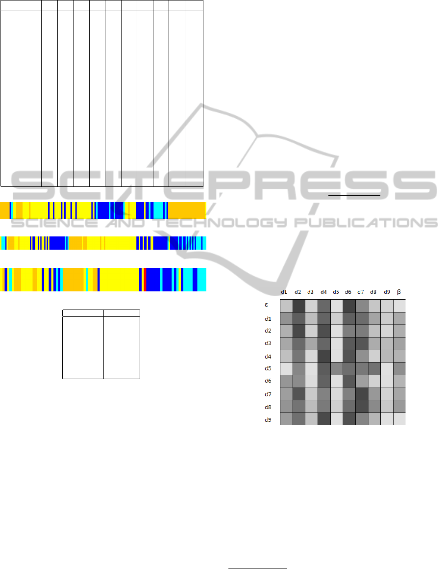
Table 4: Summary of Interests in Topics For User Commu-

nities.

Action y y y y y

Advent.

Animat. y y

Children’s

Comedy y y y y y y y y y y

Crime

Documen. y y y y y y y y y y

Drama y y y y y y y y y y

Fantasy

Noir

Horror y y y y y y y y y y

Musical

Mystery

Romance y y y

Sci-Fi

Thriller

War y y y

Western

(a)

(b)

(c)

Item Cluster Color

Red

Blue

Green

Yellow

Magenta

Orange

Cyan

Pink

Dark Grey

Figure 7: User Proﬁle Segmentation.

by the included table).

In practice, we can assume that the three users

show a common attitude towards comedy and drama,

which are the dominant topics corresponding to the

colors yellow and orange. Notice, however, that users

(b) and (c) are prone to change their interest towards

comedy, as clearly shown by the change in color.

4.4 Modeling Topic Transitions

Based on the above observations, we aim at esti-

mating the sequential connections among topics: In

practice, we would like to analyze which item cate-

gories are likely to next capture the interests of a user.

Those sequential patterns can be modeled by exploit-

ing Markov Models. The latter are probabilistic mod-

els for discrete processes characterized by the Markov

properties. We adopt a Markov Chain property here,

i.e., a basic assumption which states that any future

state only depends from the present state. This prop-

erty limits the ‘memory’ of the chain which can be

represented as a digraph where nodes represent the

actual states and edges represent the possible transi-

tions among them.

Assuming that the last observed item category for

the considered user is d

, the user could pick an item

belonging to the another topic d

with probability

p(d

). Thus, we need to estimate all the transition

probabilities, starting from a |L + 1| x |L + 1| transi-

tion count matrix T

, where T

(i, j) stores the number

of times that category j follows i in the rating proﬁle

of the users.

The estimation we provide is rather simple, corre-

sponding to a simple frequency count:

p(d

) =

(i, j)

∑

L+1

j=1

(i, j

)

Fig. 8 represents the overall transition probabil-

ity matrix, which highlights some strong connection

among given categories. As instance, the item cate-

gories having drama as dominant genre, d

, d

and d

are highly correlated as well as d

, d

and d

which

correspond to comedy movies.

Figure 8: Transition Probabilities Matrix.

It is interesting to compare how the transition

probabilities change within different user communi-

ties. Fig. 9 shows the transitions for three different

communities. Notice that, besides common transition

patterns, each community has some distinctive tran-

sitions that characterize their population. For all the

considered user communities, the most likely initial

item category is d

; while the ﬁrst and the last com-

munity reproduced in the example show a strong at-

titude corresponding to the transition d

→ d

, this is

We assume two further states ε, representing the initial

choice, and β, representing the last choice.

KDIR 2011 - International Conference on Knowledge Discovery and Information Retrieval

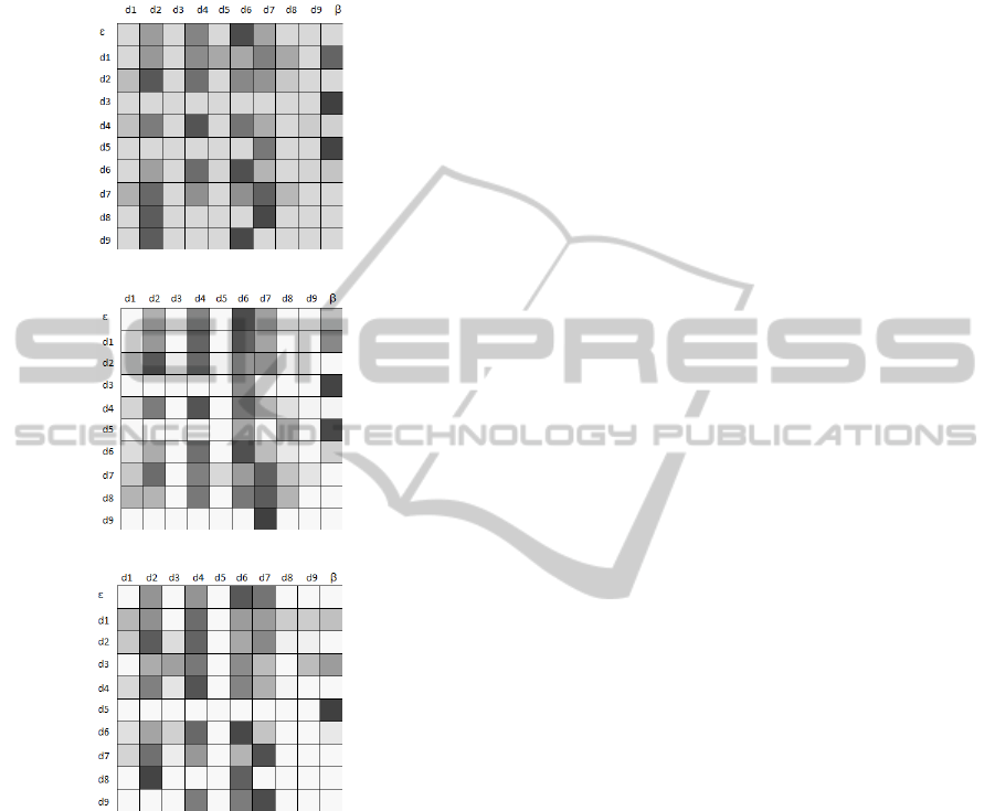
instead a weak pattern within c

. The same consider-

ation can be done for the transition d

→ d

, which is

strong for c

and c

, while users belonging to c

are

more prone to the transition towards d

(a) User community c

(b) User community c

Figure 9: Transition Probabilities Matrix.

The analysis of the transition probabilities can be

hence exploited for generating new recommendations

enforcing topic diversity (Ziegler et al., 2005) in the

top-K lists of items by taking into account not exclu-

sively the current topic of interest but the ones that

more likely could be connected to it.

5 CONCLUSIONS AND FUTURE

WORKS

In this work we focused on the application of the

Block Mixture Model to Collaborative Filtering data.

This approach allows the simultaneous clustering of

users and items and could be used to identify and mea-

sure hidden relationships among them. The proposed

model provides a ﬂexible and powerful framework to

analyze the users’ behavior. This information can be

used to improve the quality of a recommendation sys-

tem, as mentioned throughout the presentation. Fu-

ture works will focus on embedding baseline com-

ponents and normalization approaches that might be

employed to improve the quality of the clustering and

the prediction accuracy.

REFERENCES

Blei, D. M., Ng, A. Y., and Jordan, M. I. (2003). Latent

dirichlet allocation. The Journal of Machine Learning

Research, 3:993–1022.

Cremonesi, P., Koren, Y., and Turrin, R. (2010). Perfor-

mance of recommender algorithms on top-n recom-

mendation tasks. In RecSys, pages 39–46.

Funk, S. (2006). Netﬂix update: Try this at home.

George, T. and Merugu, S. (2005). A scalable collaborative

ﬁltering framework based on co-clustering. In ICDM,

pages 625–628.

Gerard, G. and Mohamed, N. (2003). Clustering with block

mixture models. Pattern Recognition, 36(2):463–473.

Govaert, G. and Nadif, M. (2005). An em algorithm for

the block mixture model. IEEE Trans. Pattern Anal.

Mach. Intell., 27(4):643–647.

Hofmann, T. and Puzicha, J. (1999). Latent class models

for collaborative ﬁltering. In IJCAI, pages 688–693.

Jin, R., Si, L., and Zhai, C. (2006). A study of mixture

models for collaborative ﬁltering. Inf. Retr., 9(3):357–

382.

Jin, X., Zhou, Y., and Mobasher, B. (2004). Web usage min-

ing based on probabilistic latent semantic analysis. In

KDD, pages 197–205.

McNee, S., Riedl, J., and Konstan, J. A. (2006). Being

accurate is not enough: How accuracy metrics have

hurt recommender systems. In ACM SIGCHI Confer-

ence on Human Factors in Computing Systems, pages

1097–1101.

Porteous, I., Bart, E., and Welling, M. (2008). Multi-hdp:

a non parametric bayesian model for tensor factoriza-

tion. In AAAI, pages 1487–1490.

Shan, H. and Banerjee, A. (2008). Bayesian co-clustering.

In ICML.

Shannon, C. E. (1951). Prediction and entropy of printed

english. Bell Systems Technical Journal, 30:50–64.

Wang, P., Domeniconi, C., and Laskey, K. B. (2009). La-

tent dirichlet bayesian co-clustering. In ECML PKDD,

pages 522–537.

Wu, H. C., Luk, R. W. P., Wong, K. F., and Kwok, K. L.

(2008). Interpreting tf-idf term weights as making

relevance decisions. ACM Trans. Inf. Syst., 26:13:1–

13:37.

Ziegler, C.-N., McNee, S. M., Konstan, J. A., and Lausen,

G. (2005). Improving recommendation lists through

topic diversiﬁcation. In WWW, pages 22–32.

CHARACTERIZING RELATIONSHIPS THROUGH CO-CLUSTERING - A Probabilistic Approach