HYBRID PARAMETER-LESS EVOLUTIONARY ALGORITHM IN
PRODUCTION PLANNING
Vida Vukaˇsinovi´c, Peter Koroˇsec and Gregor Papa
Computer Systems Department, Joˇzef Stefan Institute, Ljubljana, Slovenia
Keywords:
Production, Scheduling, Hybrid algorithm.
Abstract:
In the real-world production planning problems there are many constraints that need to be considered. Usually,
these constraints and interdependent and the optimization algorithms has to efficiently solve that. This paper
presents the hybrid parameter-less evolutionary algorithm used for construction of an optimal production plan.
The algorithm is based on genetic algorithm, but is modified to work without the parameter setting. All
algorithm control parameters are automatically determined during the optimization. The algorithm was able
to solve the constraints and to make an optimal production plan. Additionally, we evaluated the influence of
different ratios of orders with fixed deadlines on the performance of the algorithm. The used algorithm can
successfully solve also these additional constraints.
1 INTRODUCTION
Complex manufacturing processes are needed to pro-
duce various types of products. Often, each type of
similar product requires different steps, and different
product parts for completion. The effective produc-
tion plan has to allow on-time delivery, while mini-
mizing production costs in terms of overall produc-
tion time. Additionally, sometimes there are some
specific constraints to be considered, i.e., orders with
fixed deadlines. These orders have to be produced at
the exact date, which causes some other orders to be
produced either too early or with the delay. In any
case, the main problem in production processes is the
exchange delay, caused by adapting production lines
to differenttypes of products and supplying the appro-
priate parts, when switching from one type to another
on the same production line.
Several useful and efficient scheduling methods
are reported in the literature, including a genetic algo-
rithm (GA) and its variants. (Senthilkumar and Sha-
habudeen, 2006) developed a heuristic for the open
job shop scheduling problem using GA to minimize
makespan, while (Chryssolouris and Subramaniam,
2001) developed a scheduling method based on GA
and considering multiple criteria. Some other imple-
mentations of GA for job scheduling is reported by
(Vazquez and Whitley, 2000). One of the advanced
optimization techniques is a family of memetic al-
gorithms (MAs) (Ong and Keane, 2004), which rep-
resent a synergy of evolutionary approach with sep-
arate individual learning or local improvement pro-
cedures for problem search. Various MAs were de-
veloped (Caumond et al., 2008; Hasan et al., 2009)
to obtain even better results than GA. The results of
MAs not only improved the quality of solutions but
also reduced the overall computational time (Hasan
et al., 2009). Furthermore, several researchers try to
develop an algorithm that would be able to solve the
problem without human intervention for setting the
suitable control parameters (Brest et al., 2006; Harik
and Lobo, 1999). In this paper we checked the in-
fluence of the orders with fixed deadlines on the per-
formance of the advanced parameter-less implemen-
tation of GA. The problem and its solving with MA
was initially introduced in (Koroˇsec et al., 2010).
The rest of the paper is organized as follows. In
Section 2 the problem is formally defined; in Sec-
tion 3 the search approach with parameter-less algo-
rithm is described; in Section 4 the experimental en-
vironment and results are presented; and in Section 5
some conclusions are listed.
2 PRODUCTION PLANNING
Our production planning problem can be represented
as a job scheduling problem, which is NP-hard
(Brucker, 1998). A schedule is an allocation of one or
231
Vukašinovi
ˇ
c V., Korošec P. and Papa G..
HYBRID PARAMETER-LESS EVOLUTIONARY ALGORITHM IN PRODUCTION PLANNING.
DOI: 10.5220/0003085002310236
In Proceedings of the International Conference on Evolutionary Computation (ICEC-2010), pages 231-236
ISBN: 978-989-8425-31-7
Copyright
c
 2010 SCITEPRESS (Science and Technology Publications, Lda.)

more time intervals for each job to one or more ma-
chines. Let us assume we have a finite set of n jobs,
where each job consists of a chain of operations. The
jobs in our production planning problem correspond
to orders (with list of required products) and different
operations correspond to different products required
by the order. Then, we have a finite set of m machines,
where each machine can handle at most one operation
at a time. Machines correspond to production lines.
Each operation needs to be processed during an unin-
terrupted period of a given length on a given produc-
tion line. The objective is to find a schedule satisfying
certain restrictions, while minimizing the overall exe-
cution time, i.e., time for execution of all operations.
In our planning problem each production line has its
own time schedule. Further, each order has its own
deadline, which should not be missed, but can be ex-
ecuted anytime before the deadline. Each product can
be done only on some production lines and on each
of them the execution time is different. Changing the
manufacturing process from one product to another
may cause an exchange delay which depends also on
the used production line. There is also a stock. If an
operation consists of product that is in the stock then
the operation consists of using the stock and produc-
ing only missing quantity of the product. There are
several orders with fixed deadlines, which need to be
produced on the exact day, but not before.
2.1 Mathematical Formulation of the
Problem
Our production planning problem is defined by
a set of orders J = { j
1
, j
2
,..., j
n
} and a set
of production lines M = {m
1
,m
2
,...,m
m
}, where
the orders have to be processed. Each or-
der j
i
consists of a set of q
i
operations O
i
=
{(o
i1
,τ
i1
(m)),(o
i2
,τ
i2
(m)),... , (o
iq
i
,τ
iq
i
(m))}, where
o
ik
is an operation and τ
ik
(m) is its processing time de-
pended on production line used for k ∈ {1, 2,...,q
i
}.
Each operation consists of only one type of product,
therefore its processing time equals processing time
of the product p
ik
on the production line used times
number of p
ik
products. We denote a finishing time
of order j
i
by F
i
and its deadline by D
i
. Every op-
eration o
ik
of order j
i
has deadline D
i
and finishing
time F(o
ik
). Further, we denote exd(l,o
i
1
k
1
,o
i
2
k
2
) ex-
change delay between the products of operations o
i
1
k
1
and o
i
2
k
2
on production line m
l
. Notice, that the order
of o
i
1
k
1
and o
i
2
k
2
is important. By S[p
ik
] we denote the
number of products p
ik
available in the stock.
Let us assume that N is the number of operations:
N =
n
∑
k=1
|O
k
|.
A schedule is denoted by
C = g
11
g
12
g
21
g
22
···g
N1
g
N2
, (1)
where g
k1
is an index on some operation and g
k2
is
the production line used to perform operation g
k1
, for
k ∈ {1,2, . . . , N}. The task is to find the schedule, that
minimizes the number of delayed orders, exchange
delays and time to finish all the orders. The number
of delayed orders n
orders
is
n
orders
=
n
∑
i=1
delay
i
,
where
delay
i
=

0 D
i
− F
i
≥ 0
1 D
i
− F
i
< 0.
The overall exchange delay t
exd
is
t
exd
=
m
∑
l=1
N
∑
i=1
N
∑
j=i+1
δ
l,i
δ
l, j
exd(l, g
i1
,g
j1
),
where
δ
l,i
=

1 g
i2
= l (mod m)
0 otherwise.
The time to finish all the orders t
all
is
t
all
=
n
max
i=1
F
i
.
The number of days of delayed orders n
days
are
n
days
=
n
∑
i=1
delay
i
⌈(F
i
− D
i
)/(24· 60)⌉.
The constraints which also have to be considered are
the following. For the process of every o
ik
only
some production lines are appropriate. We denote
δ
ik
= (δ
m
1
,δ
m
2
,...,δ
m
m
), where
δ
ik
[l] = δ
m
l
=

1 o
ik
can be done on line m
l
0 otherwise.
Some of the orders have to be finished on exact day:
F
i
l
= D
i
l
,
for some j
i
1
, j
i
2
,..., j
i
k
∈ J and l ∈ {1,2,...,k}.
The aim is to achieve
∑
n
i=1
delay
i
= 0, but we still
allow schedule with delayed orders. The aim is also
to achieve production line equilibration, which means
we would like to minimize the finishing time differ-
ence between lines in M:
t
eq
= min
m
∑
l=1
(t
all
− FM
l
),
where FM
l
= max
N
i=1
(δ
l,i
F(g
i1
)) is maximal finishing
time on line m
l
.
ICEC 2010 - International Conference on Evolutionary Computation
232

3 HYBRID ALGORITHM
We hybridized the Parameter-Less Evolutionary
Search (PLES) (Papa, 2008) with the local search.
The PLES is based on basic GA (B¨ack, 1996; Gold-
berg, 1989), except it does not need any control pa-
rameter, e.g., population size, number of generations,
probabilities of crossover and mutation, to be set in
advance. They are set virtually, according to com-
plexity of the problem and according to statistical
properties of the solutions found. In its search pro-
cess PLES tries to efficiently explore the whole search
space in order to find the optimal solution. The hy-
bridized algorithm (PLES+LS) possesses the ability
of PLES to find a near-optimal solution in a reason-
able time, and the power of local search to move
quickly towards the optimal one.
HybridizedAlgorithm {
SetInitialPopulation(P)
Evaluate(P)
Statistics(P)
while (not EndingCondition()){
ForceBetterSolutions(P)
MoveSolutions(P)
LocalSearch()
Evaluate(P)
Statistics(P)
}
}
3.1 Population Initialization and
Termination Criterion
The production schedule was encoded into one chro-
mosome with a tuples of values, where each tuple
(gene) consisted of the index of the enumerated order
and the production line. Based on the given list of all
orders, which are sorted according to the deadlines,
various orders of indexes that represent the given or-
der are encoded in chromosome. A chromosome,
which includes encoded production schedule of n or-
ders, as presented in Equation 1.
The initial population P consists of PopSize chro-
mosomes. In each chromosome the orders are ran-
domly distributed, and also the assigned production
line is chosen randomly among possible lines for each
order. Since the numbers in the chromosome repre-
sent the indexes of orders their values can not be du-
plicated and no number can be missed; therefore both
conditions must be considered during the initializa-
tion.
The initial population size (PopSize) is set accord-
ing to the following equation
PopSize = n+ 10log
10
(
m
∑
i=1
lines
i
)
where lines
i
is the number of possible lines of the i-th
order.
The EndingCondition() function checks if there
was no improvement for several generations; then the
system was assumed to be in a steady state, and the
optimization ended. The number of generations de-
pends on the convergence speed of the best solution
found. Optimization is running while a better solu-
tion is found every few generations. But when there is
no improvement of the best solution for a few gener-
ations (Resting), the optimization process stops. The
Limit (i.e., number of generations since the last im-
provement) for stopping the optimization process is
defined as follows
Limit = 10log
10
(PopSize) + log
10
(Resting + 1)
where Resting is the number of generations since the
last improvement of the global best solution.
3.2 Variable Population Size
During the search process the population size is
changed every few generations (
Limit
5
), based on the
average change of the standard deviation of solutions
over a last few generations. When the standard devi-
ation increases than the population size is decreased,
and vice-versa. When the population is shrunk the
randomly chosen solutions are removed from the pop-
ulation, and when the population is inflated, some ran-
domly chosen solutions are duplicated.
PopSize
i
=
PopSize
i−1
Change
,
where Change is calculated as
Change =
StDev
i
+ StDev
i−1
StDev
i−1
+ StDev
i−2
.
Moreover the PopSize change is limited
to 25% per change and is further limited to
[
PopSize
5
,1.1 PopSize].
3.3 Force Better Solution
In every generation worse solutions are replaced with
better solutions, and up to 25% of genes in the chro-
mosomes are switched. This operator incorporates
(1) the function of elitism, while forcing to replace
worse solutions with better ones, and (2) the func-
tion of crossover, while taking the good solutions and
slightly change them on some positions.
HYBRID PARAMETER-LESS EVOLUTIONARY ALGORITHM IN PRODUCTION PLANNING
233

3.4 Solution Moving
Typically, every chromosome is the subject of muta-
tion in the basic GA. In PLES, mutation is performed
through the moving of some positions in the chromo-
some according to different statistical properties.
First, only the solutions that were not moved
within the ”Force better” operator are handled here.
In other words, solutions of the previous generation
that were better than the average are moved. The
number of the positions in the chromosome (Ratio)
to be moved is calculated on the basis of the standard
deviation of the solutions in the previous generation
and the maximal standard deviation as stated in the
following equation.
Ratio
i
= tanh

1−
StDev
i−1
StDev
max

× N
where StDev
i−1
and StDev
max
are the standard devi-
ation of the solution fitness of the previous genera-
tion, and the maximal standard deviation of all gen-
erations, respectively. Here Ratio ∈ {0. . . N}, and the
Ratio positions in the chromosome are selected to be
moved. The moves are implemented by changes of
production lines and/or by switching the positions of
genes in the chromosome.
3.5 Solution Evaluation and Statistics
Each population is statistically evaluated. Here the
best, the worst, and the average fitness value in the
generation are found. Furthermore, the standard de-
viation of fitness values of all solutions in the gener-
ation, the maximal standard deviation of fitness value
over all generations, and the average value of each pa-
rameter in the solution are calculated.
3.6 Local Search
Local search was implemented with four procedures,
which run sequentially.
• Stock Replacing. For each order filled from the
stock it is checked, if some other order of the same
productis scheduled for the production. If the sec-
ond one is delayed, than it is shifted in front of
the order from the stock. In this case some or-
ders of the same product are possibly moved out
of the stock and placed into the production. If the
number of the delayed orders increases, then the
shifted order is returned to its previous position.
• Deadline Sorting. For each production line, all
orders with delayed deadlines are checked if they
can be moved before some other order. The de-
layed order is moved before each of the precedent
order, so that it is not delayed anymore, while en-
suring that the total number of delayed orders is
not increased.
• Production Line Changing. For each production
line, all orders are checked if they can be placed
on any other feasible production line. If they can
be placed on some other production line, then it is
further checked if they can be merged with some
other similar order on that new production line.
The switch to another production line should not
increase the exchange delay on the new produc-
tion line.
• Similar Product Merging. For each production
line, it is checked if several orders can be merged
together. The merging is performed in four steps,
according to different properties of the products.
First the orders for the products with the same
height are merged, then those with the same size
are merged, after that the orders with the same
connectors, and finally those with the same power
characteristics. The idea of merging procedure is
to decrease the production time on each line, as
result of decreased exchange delay on the line.
3.7 Fitness Evaluation
Each new solution in the population was evaluated,
according to the number of delayed orders (n
orders
),
exchange delay times in minutes (t
exchange
), overall
production time in minutes (t
overall
), and the number
of days of delayed orders (n
days
). The cost function,
which is calculated inside Evaluate(P), is as follows:
f(P) = 10
7
· n
orders
+ 10
4
·t
exchange
+ t
overall
+ n
2
days
.
According to the cost function it is obvious that
the most important item to minimize is n
orders
, then
t
exchange
and lastly t
overall
and n
days
. The weights of
these items make sure that the first two digits of eval-
uation function value represent number of delayed or-
ders, next three digits represent exchange delay times
in minutes and the last digits represent the influence
of t
overall
and n
days
.
4 PERFORMANCE EVALUATION
4.1 The Experimental Environment
The computer platform used to perform the experi-
ments was based on AMD Athlon II
TM
2.9-GHz pro-
cessor, 4 GB of RAM, and the Microsoft
R
 Windows
R

7 operating system. The PLES+LS was implemented
in Sun Java 1.6.
ICEC 2010 - International Conference on Evolutionary Computation
234

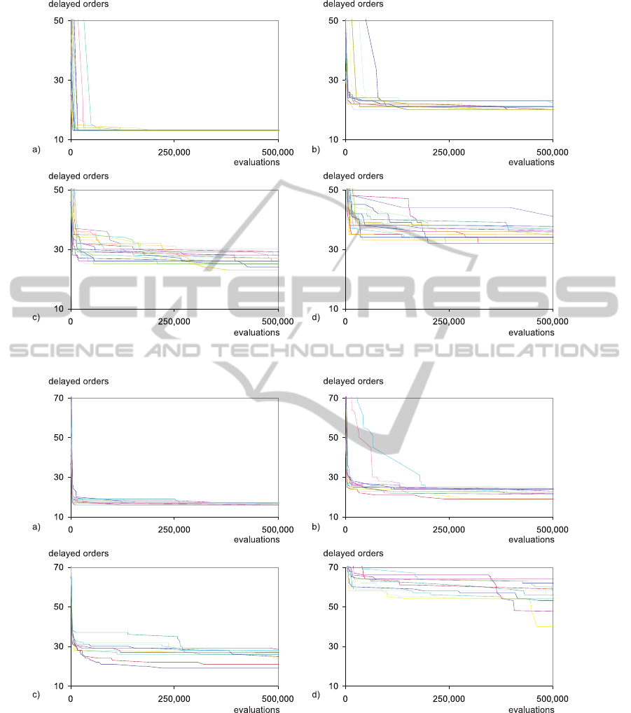
Figure 1: Influence of fixed orders on n
orders
in Task 1: a) 0%, b) 5%, c) 10%, d) 25%.
Figure 2: Influence of fixed orders on n
orders
in Task 2: a) 0%, b) 5%, c) 10%, d) 25%.
4.2 The Test Cases
The PLES+LS algorithm was tested on two differ-
ent real order lists from production company. The
first task (Task 1) consists of n = 711 orders for 251
products, while the second task (Task 2) consists of
n = 737 orders for 262 products. In both tasks the
ratio of orders with fixed deadlines varied (0%, 5%,
10%, 25%). In both tasks m = 5 production lines are
available. Each product can only be put on some pro-
duction lines (depending on the product characteris-
tics). We made 30 runs for each task, while the num-
ber of evaluations was limited to 1,000,000.
HYBRID PARAMETER-LESS EVOLUTIONARY ALGORITHM IN PRODUCTION PLANNING
235

4.3 Parameter Settings
As stated before, the control parameters are never
set in advance and are not constant. They are de-
termined each time on the basis of statistical prop-
erties of each population. Besides the population size
changes through the search progress - to enable the
search with different population sizes.
Table 1: Results of optimization for Task 1.
0% 5% 10% 25%
Best 1.314×10
8
2.017×10
8
2.316×10
8
3.227×10
8
Mean 1.319×10
8
2.037×10
8
2.561×10
8
3.417×10
8
Worst 1.325×10
8
2.117×10
8
2.819×10
8
3.738×10
8
StD 3.495×10
5
4.039×10
6
1.531×10
7
1.821×10
7
Table 2: Results of optimization for Task 2.
0% 5% 10% 25%
Best 1.616×10
8
1.934×10
8
1.837×10
8
4.054×10
8
Mean 1.663×10
8
2.149×10
8
2.381×10
8
5.051×10
8
Worst 1.723×10
8
2.421×10
8
2.833×10
8
6.249×10
8
StD 4.814×10
6
1.592×10
7
3.744×10
7
5.836×10
7
Table 3: Comparison of delayed orders.
Task 1 Task 2
0% 5% 10% 25% 0% 5% 10% 25%
Best 13 20 23 32 16 19 18 40
Mean 13 20 25 34 16 21 23 50
Worst 13 21 28 37 17 24 28 62
4.4 Results
In Tables 1 and 2 best, mean, worst, and standard de-
viations of solutions are presented for each ratio of
fixed deadlines.
To show how some of the components of the cost
function behave during the search process, we present
Figures 1 and 2. It can be visually seen, how the num-
ber of orders with fixed deadlines influences the per-
formance of PLES+LS. Here, each line represent one
run. The number of delayed orders is increasing with
the growing ratio of fixed-deadline orders.
When comparing with the previous approach
(Koroˇsec et al., 2010) of production planning, the in-
fluence of fixed orders is seen on the number of de-
layed orders. The details are presented in Table 3.
5 CONCLUSIONS AND FUTURE
WORK
In this paper, we have shown an application of spe-
cialized hybrid parameter-less evolutionary algorithm
on a real-world production planning problem. The
presence of orders with fixed deadlines influences
the performance of the hybrid PLES+LS algorithm.
However, even at 25% of orders with fixed deadlines,
the results are still better than those provided by the
expert (Koroˇsec et al., 2010).
REFERENCES
B¨ack, T. (1996). Evolutionary Algorithms in Theory and
Practice. Oxford University Press.
Brest, J., Mernik, S. G. B. B. M., and
ˇ
Zumer, V. (2006).
Self-adapting control parameters in differential evolu-
tion: A comparative study on numerical benchmark
problems. IEEE Transactions on Evolutionary Com-
putation, 10(6):646–657.
Brucker, P. (1998). Scheduling algorithms. Springer, Hei-
delberg, 2nd edition.
Caumond, A., Lacomme, P., and Tchernev, N. (2008). A
memetic algorithm for the job-shop with time-lags.
Comput. Oper. Res., 35(7):2331–2356.
Chryssolouris, G. and Subramaniam, V. (2001). Dynamic
scheduling of manufacturing job shops using genetic
algorithms. Journal of Intelligent Manufacturing,
12(3):281–293.
Goldberg, D. (1989). Genetic Algorithms in Search, Opti-
mization, and Machine Learning. Addison-Wesley.
Harik, G. and Lobo, F. (1999). A parameter-less genetic
algorithm. In Proc. Genetic and Evolutionary Com-
putation Conference (GECCO 1999), pages 258–265.
Hasan, S. M. K., Sarker, R., Essam, D., and Cornforth,
D. (2009). Memetic algorithms for solving job-shop
scheduling problems. Memetic Computing, 1(1):69–
83.
Koroˇsec, P., Papa, G., and Vukaˇsinovi´c, V. (2010). Applica-
tion of memetic algorithm in production planning. In
Bioinspired Optimization Methods and their Applica-
tions, pages 163–175.
Ong, Y. and Keane, A. (2004). Meta-lamarckian learning
in memetic algorithms. IEEE Transactions on Evolu-
tionary Computation, 8(2):99–110.
Papa, G. (2008). Parameter-less evolutionary search. In
Proc. Genetic and Evolutionary Computation Confer-
ence (GECCO’08), pages 1133–1134.
Senthilkumar, P. and Shahabudeen, P. (2006). Ga based
heuristic for the open job shop scheduling problem.
The International Journal of Advanced Manufactur-
ing Technology, 30(3-4):297–301.
Vazquez, M. and Whitley, L. D. (2000). A comparison of
genetic algorithms for the static job shop scheduling
problem. In Parallel Problem Solving from Nature,
pages 303–312. Springer.
ICEC 2010 - International Conference on Evolutionary Computation
236