
COMPUTATIONAL MODEL OF DEPTH PERCEPTION BASED ON
FIXATIONAL EYE MOVEMENTS
Norio Tagawa and Todorka Alexandrova
Faculty of System Design, Tokyo Metropolitan University, 6-6 Asahigaoka, Hino, Tokyo, Japan
Keywords:
Fixational eye movement, Depth perception, Structure from motion, Bayesian estimation, EM algorithm.
Abstract:
The small vibration of the eye ball, which occurs when we fix our gaze on an object, is called “fixational
eye movement.” It has been reported that this function works also as a clue to monocular depth perception.
Moreover, researches for a depth recovery method using camera motions based on an analogy of fixational eye
movement are in progress. We suppose that depth perception with fixational eye movement is firstly carried
out, and subsequently such depth information is supplementary used for binocular stereopsis. Especially in this
study, using camera motions corresponding to the smallest type of fixational eye movement called “tremor,”
we construct depth perception algorithm which models camera motion as a irregular perturbation, and confirm
its effectiveness.
1 INTRODUCTION
Structure from motion is typical for monocular depth
perception, and in this case an autonomous motion of
human is usually assumed. On the other hand, it is
well known that a fixational eye movement, which
means an irregular involuntary motion of eyeball,
arises when human gazes fixed targets (Martinez-
Conde et al., 2004). Since human’s retina can keep
sensitivity of receiving by finely vibrating images of
targets on a retina, fixational eye movement is the
firstly required function to watch something. The
human vision system corrects such vibration uncon-
sciously, and recognizes static images. It has been
reported that the fixational eye movement plays as
a clue for depth perception, regardless of the un-
consciousness of image motion caused by it in the
retina, and an actual vision system based on a fixa-
tional eye movement has been proposed (Ando et al.,
2002). This can suggest possibility that unconscious
depth perception is performed througha fixational eye
movement and the result is inputted into the binocular
stereopsis system with the brightness perception and
the color perception by binocular system as primitive
sources.
A lot of notable results in the study for structure
from motion (SFM) have been reported. Although
there are various computational principles for SFM,
when computatinally efficient and dense depth recov-
ery is considered to be important, the gradient method
is effective (Horn and Schunk, 1981), (Simoncelli,
1999), (Bruhn and Weickert, 2005). For the gradi-
ent method, it has to be noted that there should be an
adequate motion size for each image region in order
to recover accurate depth. Since the gradient equa-
tion can completely hold when image motion is in-
finitesimal, the equation error can not be ingored for
highly large motion. Inversely for small motion, the
motion information is hidden in observation errors of
spatio-temporal differentials of brightness, and hence
accurate depth can not be recovered. Therefore, it is
naturally required to adjust frame rate adaptively in
order to make motion size suitable. We have pro-
posed a method with no necessity of variable frame
rate, which is based on multi-resolution decomposi-
tion of images, but high computational cost is needed
(Tagawa et al., 2008). We pay attention to the small
motion so as to avoid equation error in the gradient
method. To solve the above mentioned S/N problem
caused for small motion, we should obtain many ob-
servations and use them collectively. For such strat-
egy, motion direction and motion size have to take
various values, in order to improve the accuracy inde-
pendently of the image texture.
328
Tagawa N. and Alexandrova T. (2010).
COMPUTATIONAL MODEL OF DEPTH PERCEPTION BASED ON FIXATIONAL EYE MOVEMENTS.
In Proceedings of the International Conference on Computer Vision Theory and Applications, pages 328-333
DOI: 10.5220/0002829203280333
Copyright
c
SciTePress

microsaccade
drift
tremor
Figure 1: Illustration of fixational eye movement including
microsaccade, drift and tremor.
From the above discussions, in this study, we ex-
amine a depth perception model based on fixational
eye movements. The fixational eye movement is clas-
sified into three types as shown in Fig. 1: microsac-
cade, drift and tremor. Here, we focus on the tremor,
which is the smallest one of the three types, and
construct a computation algorithm using analogy of
tremor to confirm the effectiveness of the perception
model with tremor. Since the fixational eye move-
ment is an involuntary motion, it is realistically hard
to know all of the eye movements before depth re-
covery, and thus we treat them as stochastic variables.
This problem can be realized in the framework of the
Bayesian inference, and a stable algorithm is expected
to be constructed using the EM algorithm (Dempster
et al., 1977).
2 PERCEPTION MODEL WITH
FIXATIONAL EYE MOVEMENT
As a background of this study, we are examining a
two-step perception model in which monocular depth
perception based on fixational eye movement is used
for binocular stereopsis. Binocular stereopsis plays
an essential role in the depth perception of a human
vison system (Lazaros et al., 2008), but occulusions
often occur in it. By this two-step processing, this
occulusion problem is expected to be solved. In this
study, we propose mainly a model for the first step
perception constructed additionally with the follow-
ing two-step perception
1. perception in the period of drift and tremor;
2. perception in the period of microsaccade.
In the former, depth perception corresponding to
the whole period of one drift, instead of that cor-
responding to each tremor period, is assumed to be
caused by multiple fine movements of tremor over
one period of drift. Therefore, recognized depth value
has only the temporal resolution equivalent to the pe-
riod of one drift, and has only the spatial resolution
equivalent to the distance of movement of one drift.
However, because of treating small movements, the
gradient method explained in the next section can be
used, which needs no search process and hence, is
cost effective. It should be noted that, by adopting
drift as an unit of perception, variety of brightness pat-
terns in a neigboring region can be effectively used,
and as a result accurate perception of depth can be
realized.
In the latter, using the depth value obtained by
the former step with low resolution and eye move-
ment corresponding drift, image displacement before
and after microsaccade is detected by search process
and depth value is recognized. Since the results of
the former step can be used, the size of the local re-
gion where the brightness pattern is used to search
and the range of searching area can be appropriately
determined. Additionally, because microsaccade in-
dicates fast movement, by the latter step, depth per-
ception with high spatio-temporal resolution can be
done through small computation.
As a first report of our monocular perception
model, we construct an algorithm for the first step and
confirm its efficiency. To model completely the first
step, we have to integrate drift component into the al-
gorithm, but in this study, we focus only on tremor.
Hence, we ignore the temporal correlation of tremor
which is needed to form drift component, and we as-
sume that each small movements are independent of
each other.
3 GRADIENT METHOD USING
FIXATIONAL EYE MOVEMENT
3.1 Motion Model and Optical Flow
As shown in Fig. 2, we use perspective projection as
our camera-imaging model. The camera is fixed with
an (X,Y,Z) coordinate system, where the viewpoint,
i.e., lens center, is at origin O and the optical axis is
along the Z-axis. The projection plane, i.e. image
plane, Z = 1 can be used without any loss of gen-
erality, which means that the focal length equals 1.
A space point (X,Y, Z) on the object is projected to
the image point (x,y). The camera moves with trans-
lational and rotational vectors u = [u
x
,u
y
,u
z
]
⊤
and
r = [r
x
,r
y
,r
z
]
⊤
.
We introduce a motion model representing fixa-
tional eye movement. We can set a camera’s rotation
center at the back of lens center with Z
0
along opti-
cal axis. In this study, we pick out tremor from three
COMPUTATIONAL MODEL OF DEPTH PERCEPTION BASED ON FIXATIONAL EYE MOVEMENTS
329

X
Y
Z
u
x
u
y
u
z
(x,y)
(X,Y,Z)
r
x
r
y
r
z
O
Image Plane
Object
Figure 2: Assumed projection model.
types of fixational eye movement, and hence consider
all rotations around all axes parallel with X, Y and Z
axis, respectively, as a rotation of eye ball. We repre-
sent this rotaion as r = [r
x
,r
y
,r
z
]
⊤
, and it can be used
also for the representation of the rotational vector at
origin O shown in Fig. 2. On the other hand, the trans-
lational vector u in Fig. 2 is caused by the above eye
ball’s rotation, and is formulated as follows:
u = r ×
0
0
Z
0
= Z
0
r
y
−r
x
0
. (1)
Using this representation of u and the inverse depth
d(x,y) = 1/Z(x,y), the optical flow v = [v
x
,v
y
]
⊤
is
given as follows:
v
x
= xyr
x
−(1+ x
2
)r
y
+ yr
z
−Z
0
r
y
d ≡ v
r
x
−r
y
Z
0
d,
(2)
v
y
= (1+ y
2
)r
x
−xyr
y
−xr
z
+ Z
0
r
x
d ≡ v
r
y
+ r
x
Z
0
d.
(3)
In the above equtions, d is an unknown variable at
each pixel, and u and r are unknown common param-
eters for the whole image.
3.2 Gradient Equation for Rigid Motion
The gradient equation is the first approximation of the
assumption that image brightness is invariable before
and after the relative 3-D motion between a camera
and an object. At each pixel (x,y), the gradient equa-
tion is formulated with the partial differentials f
x
, f
y
and f
t
of the image brightness f(x,y,t) and the optical
flow as follows:
f
t
= −f
x
v
x
− f
y
v
y
, (4)
where t denotes time. By substituting Eqs. 2 and 3
into Eq. 4, the gradient equation representing a rigid
motion constraint can be derived explicitly
f
t
= −( f
x
v
r
x
+ f
y
v
r
y
) −(−f
x
r
y
+ f
y
r
x
)Z
0
d
≡ −f
r
− f
u
d. (5)
In Eq. 5, f
x
, f
y
and f
t
are observations and con-
tain observation noise. Additionally, equation error,
i.e. error caused by the first approximation in Eq. 4
generally exists.
3.3 Definition of Probabilistic Model
We use M as the number of pairs of two successive
frames and N as the number of pixels. In our study,
{f
(i, j)
t
}
i=1,···,N; j=1,···,M
and {r
( j)
}
j=1,···,M
are treated
as stochastic variables, and {d
(i)
}
i=1,···,N
correspond-
ing to the inverse depth at each pixel is treated as
a definite variable and is recovered independently at
each pixel. However, since multiple frames vibrated
by irregular rotation {r
( j)
} are used for processing
and no tracking procedure is employed, to be exact
the recovered d
(i)
at each pixel does not correspond
to the value at this pixel and it takes an average value
of the neigboring region defined by vibration width in
the image. As a result, recovered d
(i)
has a correlation
with the values in the neigboring region. The spatial
extent of this correlation depends also on the depth
value, and from the begining, d
(i)
has to be treated as
the variable having such a correlation. We consider
this as a future subject.
In this study, we assume that optical flow is very
small, and hence, observation errors of f
t
, f
x
and f
y
,
which are calculated by finite difference, are small.
Additionally, equation error is also small, and there-
fore we can assume that error having no relation with
f
t
, f
x
and f
y
is added to the whole gradient equa-
tion. From this consideration, we assume that f
(i, j)
t
is a Gaussian random variable with mean 0 and vari-
ance σ
2
o
, and f
(i, j)
x
and f
(i, j)
y
have no error
p( f
(i, j)
t
|d
(i)
,r
( j)
,σ
2
o
) =
1
√
2πσ
o
×exp
−
f
(i, j)
t
+ f
r
(i, j)
+ f
u
(i, j)
d
(i)
2
2σ
2
o
. (6)
On the other hand, we also assume that r
( j)
is a 3-
dimensional Gaussian random variable with mean 0
and variance-covariancematrix σ
2
r
I, where I indicates
a 3×3 unit matrix
p(r
( j)
|σ
2
r
) =
1
(
√
2πσ
r
)
3
exp
(
−
r
( j)⊤
r
( j)
2σ
2
r
)
. (7)
From both models, the joint distribution of {f
(i, j)
t
}
and {r
( j)
} is formulated as follows:
VISAPP 2010 - International Conference on Computer Vision Theory and Applications
330

p({f
(i, j)
t
},{r
( j)
}|Θ)
=
N
∏
i=1
M
∏
j=1
p( f
(i, j)
t
|d
(i)
,r
( j)
,σ
2
o
)
M
∏
j=1
p(r
( j)
|σ
2
r
)
=
1
(2π)
M(N+3)/2
σ
MN
o
σ
3M
r
×exp
−
∑
N
i=1
∑
M
j=1
f
(i, j)
t
+ w
(i, j)⊤
r
( j)
2
2σ
2
o
−
∑
M
j=1
r
( j)⊤
r
( j)
2σ
2
r
)
, (8)
w
(i, j)
=
f
(i, j)
x
x
(i)
y
(i)
+ f
(i, j)
y
(1+ y
(i)
2
)
−f
(i, j)
x
(1+ x
(i)
2
) − f
(i, j)
y
x
(i)
y
(i)
f
(i, j)
x
y
(i)
− f
(i, j)
y
x
(i)
+Z
0
d
(i)
f
(i, j)
y
−f
(i, j)
x
0
≡ w
(i, j)
0
+ Z
0
d
(i)
w
(i, j)
d
, (9)
where Θ = {{d
(i)
},σ
2
o
,σ
2
r
}. Additionally, the poste-
rior distribution of {r
( j)
} is
p({r
( j)
}|{f
(i, j)
t
},Θ) =
p({r
( j)
},{f
(i, j)
t
}|Θ)
p({f
(i, j)
t
}|Θ)
, (10)
and this can be arranged as the following Gaussian
distribution
p({r
( j)
}|{f
(i, j)
t
},Θ) =
1
q
(2π)
3M
∏
M
i=1
detV
( j)
r
×exp
(
−
1
2
M
∑
j=1
r
( j)
−r
( j)
m
⊤
V
( j)
r
−1
r
( j)
−r
( j)
m
)
,
(11)
where
r
( j)
m
= −
1
σ
2
o
V
( j)
r
N
∑
i=1
f
(i, j)
t
w
(i, j)
, (12)
V
( j)
r
=
1
σ
2
o
N
∑
i=1
w
(i, j)
w
(i, j)⊤
+
1
σ
2
r
I
!
−1
. (13)
3.4 Computation Algorithm
In order to determine Θ as a maximum likelihood esti-
mator and to determine {r
( j)
}as a MAP estimator, we
apply the EM algorithm by treating {{f
(i, j)
t
},{r
( j)
}}
as a complete data and {r
( j)
} as a missing data.
The log likelihood function of the complete data
l
c
(Θ) is derived from Eq. 8 as
l
c
(Θ) = Const. −
MN
2
lnσ
2
o
−
3M
2
lnσ
2
r
−
1
2σ
2
o
N
∑
i=1
M
∑
j=1
f
(i, j)
t
+ w
(i, j)⊤
r
( j)
2
−
1
2σ
2
r
M
∑
j=1
r
( j)⊤
r
( j)
= Const. −
MN
2
lnσ
2
o
−
3M
2
lnσ
2
r
−
1
2σ
2
o
M
∑
j=1
(
N
∑
i=1
f
(i, j)
t
2
+ 2
N
∑
i=1
f
(i, j)
t
w
(i, j)⊤
!
r
( j)
+tr
"
N
∑
i=1
w
(i, j)
w
(i, j)⊤
!
r
( j)
r
( j)⊤
#)
−
1
2σ
2
r
M
∑
j=1
tr
r
( j)
r
( j)⊤
. (14)
In the EM algorithm, the E step and the M step
are mutually repeated until they converge. At first,
in the E step, the conditional expectation of the log
likelihood with observing {f
(i, j)
t
}, which is called Q
function, is computed. In the Q function, the esti-
mated value
ˆ
Θ is used for the parameters values in the
conditional distribution. In the following, the values
computed using
ˆ
Θ are indicated as ˆ·. Taking expecta-
tion of Eq. 14 results in expectation of the terms con-
taining {r
( j)
}, and using
E
h
r
( j)
i
≡
ˆ
r
( j)
m
(15)
and
E
h
r
( j)
r
( j)⊤
i
≡
ˆ
R
( j)
=
ˆ
V
( j)
r
+
ˆ
r
( j)
m
ˆ
r
( j)
m
⊤
, (16)
and ignoring constant value, the Q function becomes
Q(Θ) = −
MN
2
lnσ
2
o
−
3M
2
lnσ
2
r
−
1
2σ
2
o
M
∑
j=1
(
N
∑
i=1
f
(i, j)
t
2
+ 2
N
∑
i=1
f
(i, j)
t
w
(i, j)⊤
!
ˆ
r
( j)
m
+tr
"
N
∑
i=1
w
(i, j)
w
(i, j)⊤
!
ˆ
R
( j)
#)
−
1
2σ
2
r
M
∑
j=1
tr
ˆ
R
( j)
.
(17)
In the M step, Θ is updated so as to maximize the
Q function. We rewrite Eq. 17 as follows:
Q(Θ) = −
MN
2
lnσ
2
o
−
3M
2
lnσ
2
r
−
1
2σ
2
o
ˆ
F({d
(i)
}) −
1
2σ
2
r
ˆ
G. (18)
From this representation, σ
2
o
and σ
2
r
can be updated as
σ
2
o
=
ˆ
F({d
(i)
})
MN
, σ
2
r
=
ˆ
G
3M
. (19)
COMPUTATIONAL MODEL OF DEPTH PERCEPTION BASED ON FIXATIONAL EYE MOVEMENTS
331
Additionally, {d
(i)
} can be also updated as follows:
d
(i)
=
−
∑
M
j=1
f
(i, j)
t
w
(i, j)
d
⊤
ˆ
r
( j)
m
+ tr
B
(i, j)
ˆ
R
( j)
Z
0
∑
M
j=1
tr
A
(i, j)
ˆ
R
( j)
,
(20)
where the matrices A
(i, j)
and B
(i, j)
are defined as
A
(i, j)
≡ w
(i, j)
d
w
(i, j)
d
⊤
, (21)
B
(i, j)
≡
w
(i, j)
d
w
(i, j)
0
⊤
+ w
(i, j)
0
w
(i, j)
d
⊤
2
. (22)
4 NUMERICAL EVALUATIONS
To confirm the effectiveness of the proposed method,
we conducted numerical evaluations using artificial
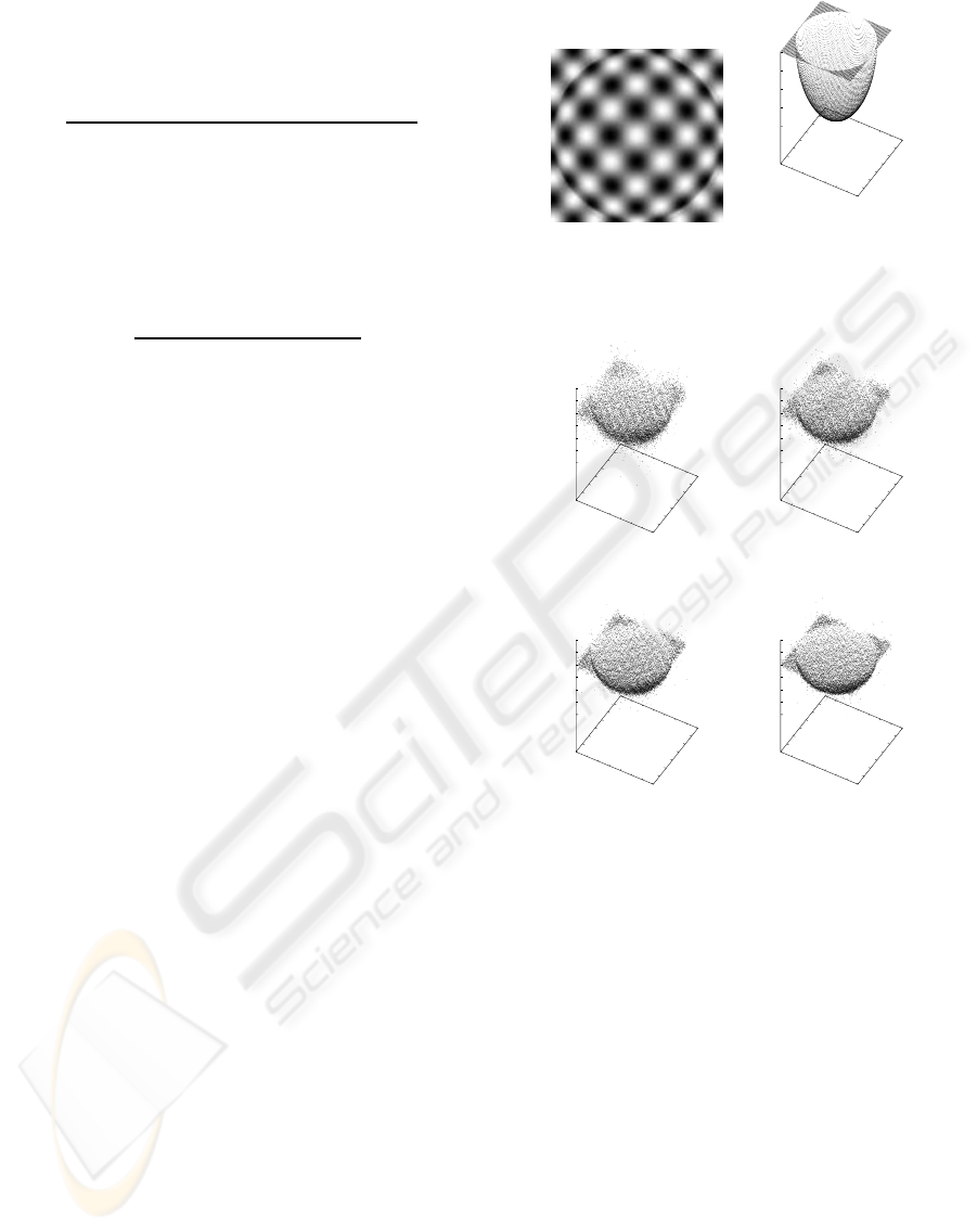
images. Figure 3(a) shows the original image gener-
ated by a computer graphics techniqueusing the depth
map shown in Fig. 3(b). The image size assumed in
these evaluations is 128×128 pixels. In Fig. 3(b), the
vertical axis indicates the depth Z and the horizontal
axes means (x,y) in the image plane.
In our model, pairs of two successive images are
assumed to be used in turn to calculate f
t
. For this
model, we have to adjust the correlation between suc-
cessive rotations in order to keep the movement range
at each image position in a certain local region, other-
wise each position may move divergently as a random
walk model. In these evaluations, to simplify the pro-
cedures, each rotation value was generated as a Gaus-
sian independent random variable by computer, and
the pairs to define f
t
were taken as the original image
and each successive image. Additionally, in order to
firstly justify our algorithm for the assumed statistical
models, we computed {f
t
} using Eq. 5 with the true
value of r and {d} and use them for depth recovery.
Figure 4 shows examples of the recovered depth
map. The random value of each component of r was
generated as a Gaussian random variable with mean 0
and deviation 0.01 [rad./frame]. Under this condition,
the mean magnitude of optical flow took the value be-
tween one and two pixels. These results shown in
Fig. 4 were calculated from {f
t
} having noise. A
Gaussian random values with mean 0 and deviation
corresponding to 1% of the deviation of the true {f
t
}
were added to the true {f
t
}. The initial value of both
σ
2
o
and σ
2
r
was 1.0 ×10
−2
as an arbitrary value, and
{d} was assumed initially as a plane of Z = 9.0. By
varying the value of M corresponding to the number
of sets {f
t
} between 100 and 800, we confirmed the
(a) (b)
0
20
40
60
80
100
120
140
0
20
40
60
80
100
120
140
8
8.5
9
9.5
10
Figure 3: Example of the data used in the experiments: (a)
artificial image used as an original image for making the
successive images; (b) true depth map used for generating
the images.
(a)
0
20
40
60
80
100
120
140
0
20
40
60
80
100
120
140
6
7
8
9
10
11
12
(b)
0
20
40
60
80
100
120
140
0
20
40
60
80
100
120
140
6
7
8
9
10
11
12
(c)
0
20
40
60
80
100
120
140
0
20
40
60
80
100
120
140
6
7
8
9
10
11
12
(d)
0
20
40
60
80
100
120
140
0
20
40
60
80
100
120
140
6
7
8
9
10
11
12
Figure 4: Stability of the proposed model for 1% noise of
f
t
: (a) M = 100; (b) M = 200; (c) M = 400; (d) M = 800.
effectiveness of collective utilization of many obser-
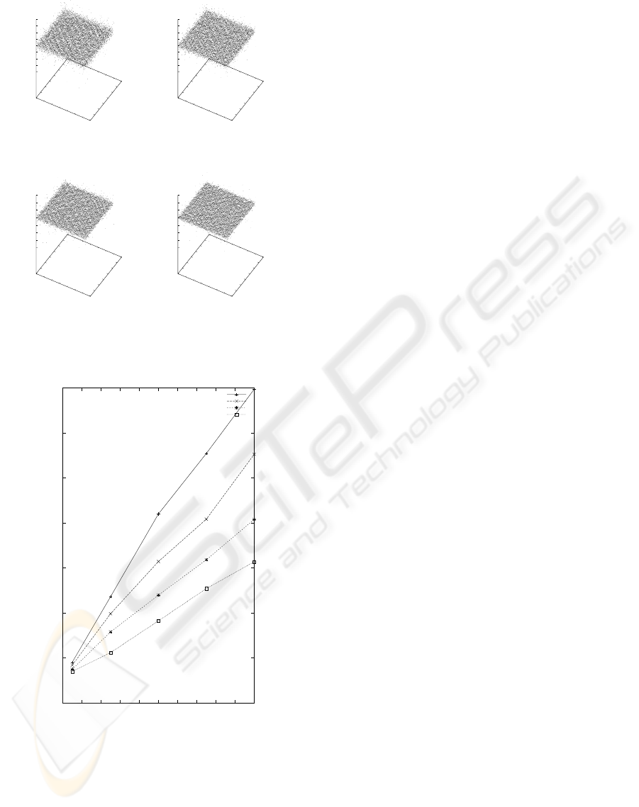
vations. The error maps of the recovered depth maps
are also shown in Fig. 5. Additionally, the RMSEs
of the recovered depth with respect to the noise de-
viation of {f
t
} are shown in Fig. 6. The outliers of
the recovered depth taking the value below 6 or over
12 were excluded for evaluation of the RMSEs. From
these results, we can conclude that the observations
collection works well for accurate recovery.
5 CONCLUSIONS
In this paper, we propose a depth perception model
with fixational eye movements. Especially for tremor,
we construct a computation algorithm which recovers
depth at each pixel collectively using multiple images
overthe period of one drift. Since this algorithm treats
VISAPP 2010 - International Conference on Computer Vision Theory and Applications
332
(a)
0
20
40
60
80
100
120
140
0
20
40
60
80
100
120
140
-4
-3
-2
-1
0
1
2
3
4
(b)
0
20
40
60
80
100
120
140
0
20
40
60
80
100
120
140
-4
-3
-2
-1
0
1
2
3
4
(c)
0
20
40
60
80
100
120
140
0
20
40
60
80
100
120
140
-4
-3
-2
-1
0
1
2
3
(d)
0
20
40
60
80
100
120
140
0
20
40
60
80
100
120
140
-4
-3
-2
-1
0
1
2
3
Figure 5: Error map corresponding to the recovered depth
shown in Fig. 4: (a) M = 100; (b) M = 200; (c) M = 400;
(d) M = 800.
0
0.1
0.2
0.3
0.4
0.5
0.6
0.7
0 0.2 0.4 0.6 0.8 1 1.2 1.4 1.6 1.8 2
RMSEs of depth
Noise dev. of ft [%]
M = 100
M = 200
M = 400
M = 800
Figure 6: RMSEs of recovered depth with respect to noise
deviation of f
t
by varying M.
small changes of image brightness pattern, the linear
approximation error contained in the gradient equa-
tion becomes small. Moreover, because one depth
map corresponding to multiple successive images is
recoved, the bad influence of observation errors can
be reduced.
In future, in order to get an accurate depth map
with small successive images, we are going to exam-
ine a model in which depth values in the local region
are assumed to be constant or to have spatial correla-
tion. Additionally, we have to construct whole algo-
rithm based on fixational eye movementand binocular
stereopsis, and have to show the effectiveness of the
algorithm through the real image experiments.
REFERENCES
Ando, S., Ono, N., and Kimachi, A. (2002). Involuntary
eye-movement vision based on three-phase correla-
tion image sensor. In proc. 19th Sensor Symposium,
pages 83–86.
Bruhn, A. and Weickert, J. (2005). Locas/kanade meets
horn/schunk: combining local and global optic flow
methods. Int. J. Comput. Vision, 61(3):211–231.
Dempster, A. P., Laird, N. M., and Rubin, D. B. (1977).
Maximum likelihood from incomplete data. J. Roy.
Statist. Soc. B, 39:1–38.
Horn, B. K. P. and Schunk, B. (1981). Determining optical
flow. Artif. Intell., 17:185–203.
Lazaros, N., Sirakoulis, G. C., and Gasteratos, A. (2008).
Review of stereo vision algorithm: from software to
hardware. Int. J. Optomechatronics, 5(4):435–462.
Martinez-Conde, S., Macknik, S. L., and Hubel, D. (2004).
The role of fixational eye movements in visual percep-
tion. Nature Reviews, 5:229–240.
Simoncelli, E. P. (1999). Bayesian multi-scale differential
optical flow. In Handbook of Computer Vision and
Applications, pages 397–422. Academic Press.
Tagawa, N., Kawaguchi, J., Naganuma, S., and Okubo, K.
(2008). Direct 3-d shape recovery from image se-
quence based on multi-scale bayesian network. In
proc. ICPR ’08, pages CD–ROM.
COMPUTATIONAL MODEL OF DEPTH PERCEPTION BASED ON FIXATIONAL EYE MOVEMENTS
333
