ON USING SIMULATION AND STOCHASTIC LEARNING FOR

PATTERN RECOGNITION WHEN TRAINING DATA IS

UNAVAILABLE

The Case of Disease Outbreak

Dragos Calitoiu

and B. John Oommen

1, 2

School of Computer Science, Carleton University, 1125 Colonel By Drive, Ottawa, Canada

Department of Information and Communication Technology

University of Agder, 36 Grooseveien, Grimstad, Norway

Keywords:

Disease outbreak, Stochastic point location, Learning automata.

Abstract:

Pattern Recognition (PR) involves two phases, a Training phase and a Testing Phase. The problems associated

with training a classiﬁer when the number of training samples is small are well recorded. Typically, the

matrices involved are ill-conditioned and the estimates of the probability distributions are very inaccurate,

leading to a very poor classiﬁcation system. In this paper, we report what we believe are the pioneering results

for designing a PR system when there are absolutely no training samples. In such a scenario, we show how

we can use a model of the underlying phenomenon and combine it with the principle of stochastic learning

to design a very good classiﬁer. By way of example, we consider the case of disease outbreak: Learning the

Contagion Parameter in a black box model involving healthy, sick and contagious individuals. The parameter

of interest involves η which is the probability with which an infected person will transmit the disease to a

healthy person. Using the theory of Stochastic Point Location (SPL), the problem is reduced to a PR or

classiﬁcation problem in which the SPL is ﬁrst subjected to a training phase, the outcome of which is used for

the testing phase.

1 INTRODUCTION

The Training phase of every PR problem is, in one

sense, the most difﬁcult. It ﬁrst of all involves un-

derstanding the type of classiﬁer that is to be used.

Once this is determined, the various class-conditional

distributions have to be learned, and this incorpo-

rates all the facets of learning. Indeed, it is so all-

pervasive that almost all of PR considers how training

can be achieved for parametric/non-parametric data,

for different distributions and when one encounters

the “curse of dimensionality”. But in every case, the

basic premise is that the designer is given a reasonable

number of training samples. Of course, every prac-

titioner would like an “inﬁnite” number of training

samples, because then, everything converges beauti-

fully. The problems associated with training a classi-

ﬁer when the number of training samples is small, are

well recorded. In such cases, the matrices involved

are ill-conditioned and the estimates of the probabil-

ity distributions are very inaccurate, implying that the

classiﬁcation system is very poor.

In this paper, we consider how we can design a PR

system when we have no training samples. Although

such cases are rare, they are extremely important. In-

deed, policy-related decisions concerning the spread

of infectious diseases always involve phenomena that

have almost never been encountered before. In a cer-

tain disease outbreak, we show how we can use a

model of the underlying phenomenon and combine

it with the principles of stochastic learning to design

a very good classiﬁer. As far as we know, the entire

process of designing PR systems and training them in

such situations is open, and thus, we believe that the

results we present are, in one sense, pioneering. To

clarify issues, rather than dealing with a PR problem

in an abstract domain, we shall consider how PR can

be achieved in the so-called “Learning the Contagion

Parameter” (LCP) problem.

As a preface, we ﬁrst present the environment

against which the LCP problem must be studied and

the proposed solution utilized. We assume that we are

dealing with a geographical area of ﬁxed dimensions

which could represent a certain district of a city. In the

Calitoiu D. and John Oommen B. (2010).

ON USING SIMULATION AND STOCHASTIC LEARNING FOR PATTERN RECOGNITION WHEN TRAINING DATA IS UNAVAILABLE - The Case of

Disease Outbreak.

In Proceedings of the 2nd International Conference on Agents and Artiﬁcial Intelligence - Artiﬁcial Intelligence, pages 45-52

DOI: 10.5220/0002716800450052

 SciTePress

interest of simplicity the population of this area is as-

sumed constant. When an infection starts within this

geographical area it is desirable, ﬁrst of all, that the

contagion is contained within the area. The second is-

sue which is primarily of concern to our present study

involves understanding how the disease can spread to

healthy people within this geographical area. In other

words, we would like to determine when the outbreak

of the disease is under control, and also to be able to

detect an uncontrollable explosion - which are the re-

spective classes in our PR problem. Once we are able

to detect these scenarios, it will be the task of the pol-

icy makers to propose strategies by which quarantine

decisions are made. This present study and the pro-

posed results, hopefully, submit a small step in this

direction. To present the problem in the right perspec-

tive, we submit a brief explanation of the disease out-

break problem and the epidemiological model used.

1.1 The Disease Outbreak Problem

A disease outbreak is commonly deﬁned as the occur-

rence of an illness in a community or region, where

the number of cases of the illness occur with a fre-

quency clearly in excess of normal expectancy. The

number of cases indicating the presence of an out-

break will vary according to the infectious agent, size

and type of the population exposed, previous experi-

ence or lack of exposure to the disease, and the time

and place of the occurrence(s). Thus, the status of

an outbreak is relative to the usual frequency of the

disease in the same area, among the same population,

and at the same season of the year (Chin, 2000).

In outbreak situations, one often must introduce

preventive interventionsto control pathogen transmis-

sion and adverse outcomes. Control measures that

have proven effective in similar outbreaks in the past

can thus be immediately implemented.

Conﬁrming an outbreak begins with the calcula-

tion of the background rate of infection (or adverse

event) and then comparing the outbreak period rate

with the background rate. Such a comparison can be

performed using the rate ratio (R

Attack rate during epidemic period

Attack rate during background period

(1)

An outbreak become uncontrollablewhen the pro-

posed control measures are not able to keep the rate

ratio constant or, to decrease it.

The models are used by policymakers, public

health workers, and other researchers who want to an-

alyze and compare the outcomes to better understand

how an outbreak occurs, and how a disease spreads.

They are also useful for understandinghowto respond

to emerging infectious diseases. If a disease outbreak

occurs, simulations can be done by tuning speciﬁc

models to aid public ofﬁcials in their decision-making

processes.

Our method is an alternative approach to the fol-

lowing two classical methods, namely, a Sensitiv-

ity Analysis and Monte Carlo Investigations, respec-

tively.

Sensitivity analysis estimates what the true effect

measure (e.g., the rate ratio) would be in the light of

the observed data and a hypothetical level of bias. It

produces one or more hypothetically adjusted point

estimates for the speciﬁc measure of interest (Green-

land, 1998).

Monte Carlo investigations, (i.e., at least in the

present context), involve the simulation of real phe-

nomena, or their idealized models, involving a ran-

dom or probabilistic element in their structure, by the

deliberate use of random numbers. These methods

have already played an important role in many appli-

cations of stochastic models and processes, both by

way of background material (in understanding quali-

tatively some of the properties of such models), and

more quantitatively, in the study of particular prob-

lems that are not amenable to complete mathematical

solution (Robert and Casella, 2005).

We propose a new methodology to investigatehow

an outbreak occurs, which possesses an advantage of

less computational effort compared with the above-

mentioned approaches.

1.2 Principles of Contagion

Epidemiology is the study of the spread of any dis-

ease, with regard to space and time. Its objective is to

trace the factors and parameters that are responsible

for, or contribute to, their occurrence (Diekmann and

Heesterbeek, 2000).

In the process of studying the spread of a disease,

the spatial structure of a population, its density and

the geographical area involved can have a major con-

tribution. As opposed to this, the non-spatial mathe-

matical models can provideonly a simple image about

the dynamics of the transmission. Consequently, this

requires, in many situations, more realistic models

that include the description of the space and the spa-

tial contact between individuals. The basic idea of

studying the dynamics of spreading a disease is to

distinguish individuals from one another according to

their features, their interaction with the environment,

and involves discovering the variation in time of these

features. In the case of an infectious disease, the prin-

cipal characteristic is the computation of the “force”

of infection of a given agent that modiﬁes the state of

ICAART 2010 - 2nd International Conference on Agents and Artificial Intelligence

an individual (Diekmann and Heesterbeek, 2000).

The state of the individual is speciﬁed with the

minimal “degree of freedom” so that we can ade-

quately predict the future of the individual from an

epidemiologic point of view. We attempt to describe

the state of the population and nature, symbolically

given as S(t + 1) at time ‘t + 1’, be only a function

of S(t). The evolution uses the assumption that the

state S(t) completely captives the history of what hap-

pened prior to the time instant, ‘t’, as per the so-called

Markovian assumption. Also, the simplest epidemic

models assume that any pair of individuals is equally

likely to interact with each other during a given time

interval. This is referred to as the well-mixed assump-

tion.

In our research, we investigate the problem of

learning the Contagion Parameter (CP) in the process

of transmission and perpetuation of a virus in a (hu-

man) population, by using the so-called regular lat-

tice model.

A classical example of such a model for conta-

gion simulates the transmission of a virus in a human

population. The model is initialized with N people,

of which I are infected at time ‘t’. People move ran-

domly about the lattice, being either (i) healthy but

susceptible to infection (S), (ii) sick and infectious (I),

(iii) recovered and immune (R), or (iv) dead (D). We

do not allow for individual to reproduce or enter in the

geographical area, implying that N=S+I+R+D.

The density of the population also affects how

often infected, immune and susceptible individuals

come into contact with each other. To render the

model tractable, we assume that infection leads to ei-

ther death due to the illness or immunity. Thus, no

individual can be infected twice. Additionally, we

model the system with the understanding that contam-

ination can take place when two individuals, either of

whom is sick, make “contact” with each other. This

is characterized by the probability that a contact be-

tween a contagious and a susceptible person actually

leads to transmission. This is symbolized by the Con-

tagion Parameter (CP), η, assumed to be constant

but unknown. Finally, the period of the infection is the

same for all individuals. Thus, the infectivity quanti-

ﬁes the probability that the transmission of the illness

will occur when a contagiousand a susceptible person

occupy the same physical grid location.

1.3 Formal Model of Contagion

Solving the problem in its absolute generality - even

from a modeling perspective - is probably intractable.

To render this problem tractable, obviously, we have

to resort to some simplifying assumptions listed be-

low.

Assumption A1: We assume that we are working

within a square grid of width W units.

Assumption A2: We assume that there are N, con-

stant, individuals moving in this grid in a locally ran-

domized manner. The number of sick people at time

‘t’ is given by n

(t).

Assumption A3: We assume that we are working in a

discretized time space, t = 1···t

max

where t

max

is the

total period of observation.

Assumption A4: We consider a scale-independent

model.

Assumption A4.1: First of all, the number of indi-

vidual is speciﬁed in term of a density coefﬁcient ρ,

where ρ =

Assumption A4.2: The number of the sick people at

any time ‘t’, namely n

(t), will be determined by the

ratio σ, where σ(t) =

(t)

Assumption A5: We assume that every individual C

is characterized by a 4-tuple hx

(t), y

(t), s

, d

i where,

at any time instant t,

Assumption A5.1: x

, y

∈ {1···W} (i.e. the condi-

tions of the location of the individual).

Assumption A5.2: s

is an indicator signifying the

state of the individual C

. By convention, a healthy

person is assigned the index s

= 0. He is sick if s

= 1,

immune if s

= 2, and dead if s

= 3.

Assumption A5.3: d

is the duration of time that has

elapsed since the instant when the value s

was set to

unity. It represents the time that has elapsed since the

sick individual was infected.

Assumption A6: At every time instant the individual

is permitted to move to one of his neighboring grid

locations or to stay where it is. We assume that the

individual stays at its current location with the prob-

ability θ (assumed to be ﬁxed and known, and moves

to one of its neighboring locations with the probabil-

ity

1−θ

, where K is the number of cells which are

neighboring to hx

, y

Assumption A7: Every individual can infect another

with a probability η which is the unknown parameter

within the simpliﬁed model of contagion.

Assumption A8: Every sick individual can either die

or become immune to the illness after a period, τ, also

referred to as the Period of Infectivity. Only during

this period he is capable of infecting a healthy person.

With the above assumptions, we ﬁrst formalize

the model. We assume that N individuals are mov-

ing within the grid of width W, and that at every time

instant each individual is allowed to stay or move to

a neighboring cell as per Assumption A6. Whenever

two individuals are on the same grid point, the con-

tagion possibilities are three-fold: (i) If both the in-

dividuals are healthy they remain healthy. (ii) If both

ON USING SIMULATION AND STOCHASTIC LEARNING FOR PATTERN RECOGNITION WHEN TRAINING

DATA IS UNAVAILABLE - The Case of Disease Outbreak

the individuals are infected, they continue to be in-

fected. (iii) If exactly one of them is sick, he contami-

nates the other with the probability η. Based on these

assumptions, since ρ is the density of the number of

individuals and σ

is the proportion

of sick people

(among the entire population) at time t, σ

t+1

has the

following form: σ

t+1

= f(σ

, ρ, η), where the func-

tional form of f(·) is unknown. Our aim is, quite sim-

ply, to achieve the PR on the process, which in turn

implies estimating η, and we achieve this by using a

learning methodology applied to solve the Stochastic

Point Location (SPL) problem.

2 STOCHASTIC POINT

LOCATION

The SPL problem (Oommen, 1997; Oommen and

Raghunath, 1998; Oommen et al., 2006) considers a

general learning problem in which the learning mech-

anism (which could be a Learning Automaton (LA),

or in general, an algorithm) attempts to learn a “pa-

rameter”, say η

∗

, within a closed interval. Consider

the problem of a robot moving around on a real line

attempting to locate a particular point. To assist the

mechanism, it communicates with an Environment

which provides it with information regarding the di-

rection in which it should go. If the Environment is

deterministic, the problem is the “Deterministic Point

Location Problem”.

This problem is akin to the ﬁeld of LA (Laksh-

mivarahan, 1981; Narendra and Thathachar, 1989;

Poznyak and Najim, 1997; Thathachar and Sastry,

2003), in which the learning mechanism attempts to

learn from a stochastic Teacher. More speciﬁcally,

unlike the traditional LA model in which the LA at-

tempts to learn the optimal action offered by the En-

vironment, we consider the following learning prob-

lem: the learning mechanism is trying to locate an un-

known point on a real interval by interacting with the

stochastic Environment through a series of informed

guesses.

Unlike the deterministic problem alluded to

above, in the SPL, rather than receive deterministic

responses as to where it should go, the learning mech-

anism is given, at every time step, a stochastic (i.e.,

possibly erroneous) response. Thus, when it should

really be moving to the “right” it may be advised to

move to the “left” and vice versa, as formalized be-

low.

In the interest of readability, for all time instants, σ

will be used to represent σ(t).

2.1 Formulation of the SPL Problem

We assume that there is a learning mechanism whose

task is to determine the optimal value of some vari-

able (or parameter), η. We assume that there is an op-

timal choice for η - an unknown value, say η

∗

∈ [0, 1].

The question which we study here is the one of learn-

ing η

∗

. Although the mechanism does not know the

value of η

∗

, we assume that it has responses from an

intelligent “Environment” E which is capable of in-

forming it whether the current value of η is too small

or too big. E may tell us to increase η when it should

be decreased, and vice versa. However, to render the

problem tangible we assume that the probability of

receiving an intelligent response is p > 0.5.

Observe that the quantity “p” reﬂects on the “ef-

fectiveness” of the Environment, E. Thus, whenever

the current η < η

∗

, the Environment correctly sug-

gests that we increase η with probability p. It simulta-

neously could have incorrectly recommended that we

decrease η with probability (1 − p). Similarly, when-

ever η > η

∗

, the Environment tells us to decrease η

with probability p, and to increase it with probability

(1− p).

We shall assume that η is any number in the in-

terval [0, 1]. The question of generalizing thus will be

considered later. The crucial issue that we have to ad-

dress is that of determining how to change our guess

of η

∗

in [0, 1]. We shall attempt to do this in a dis-

cretized manner by subdividing the time unit interval

into R steps {0,

, ...,

R−1

, 1}, where R is the reso-

lution of the learning scheme. A larger value of R will

ultimately imply a more accurate convergence to the

unknown η

∗

The scheme which attempts to learn η

∗

is as be-

low. Let η(t) be the value at time step “t”. Then,

η(t + 1) := η(t) +

, (2)

if E suggests increasing η and 0 ≤ η(t) < 1;

η(t + 1) := η(t) −

, (3)

if E suggests decreasing η and 0 < η(t) ≤ 1.

At the end states, the scheme obeys:

η(t + 1) := η(t), (4)

if η = 1 and E suggests increasing η;

η(t + 1) := η(t), (5)

if η = 0 and E suggests decreasing η.

The Markov Chain representing these transitions

is given in Figure 1 below.

Notice that although the above rules are determin-

istic, because the “environment” is assumed faulty,

ICAART 2010 - 2nd International Conference on Agents and Artificial Intelligence

Figure 1: The Markov Chain used for solving the SPL.

The states are represented here by integers in {0,1,2,..., R},

where state i represents a value of η =

the state transitions are stochastic. The main result

concerning the above scheme is the following:

Theorem. The parameter learning algorithm speci-

ﬁed by Equations (2)-(5) is asymptotical optimal.

The proof of the theorem can be found in (Oom-

men et al., 2008).

3 USING SPL FOR LEARNING

THE CP AND TO ACHIEVE PR

This section describes the strategy by which the so-

lution to the SPL will be used to learn the CP of the

contagion model. In essence, we shall reduce this to a

Pattern Recognition (PR) problem, and thus, this will

consist of two phases: a Training phase and a Testing

phase. The Training phase can be considered to be a

calibration module, which essentially learns how an

arbitrary disease will spread under the constraints of

our model. This can be obtained in a completely non-

real-life setting because we need to understand how

the number of sick individuals at any time is related

to the number of sick individuals at the prior time in-

stant, the density, ρ, and the contagion parameter, η.

The Testing phase would then involve dealing with

the sick individuals in the real life or simulated set-

ting, and attempting to estimate η. We now discuss

both of these phases.

3.1 The Training Phase

We shall ﬁrst explain the principle used in Training,

and then illustrate the results of the training that we

have achieved.

As mentioned in the modeling phase, since ρ is

the density of the number of individuals and σ

is the

proportion of sick people (among the entire popula-

tion) at time t, σ

t+1

has the following form: σ

t+1

f(σ

, ρ, η). Clearly, the functional form of f is un-

known, and it is our task to ﬁrst of all learn it, and to

secondly, use the learned form in the inference prob-

lem associated with learning what the true CP, η

∗

is.

The Training is achieved by explicitly invoking

the functional interdependence of σ

t+1

on σ

. This

will, in turn, be achieved by allowing the individu-

als, to move and contaminate/recover from the ill-

ness as per the model speciﬁed earlier. Thus, the

training phase can be given by the following algo-

rithm, formally described below in Algorithm Train-

ing Phase.

Assumptions: The algorithm is able to move the

location of an individual as per Assumption A6.

This is achieved by invoking the function Move.

Input:

W: The size of the grid, which is assumed to be a

square W ×W.

N: The number of individuals in the grid.

θ: The probability of an individual not moving in

the grid.

: The number of initial sick individuals.

η: The probability of infection.

τ: The Period of Infectivity.

: The Probability of Recovery

Output:

The updated n

as a function of ρ, the density of the

population and η.

BEGIN Algorithm Training Phase

Initialize every C

= hx

, y

, s

, d

i to a random posi-

tion x

, y

Set the value of s

to be 1 with the proportion deter-

mined by N, ρ, and n

(0).

is initialized to zero for every individual.

repeat forever

/*Compute the position for each individual*/

for i=1 to N do

(t + 1), y

(t + 1)i := Move[hx

(t), y

(t)i, θ];

end for

/*Compute the sick state for each individual*/

for i=1 to N do

if (s

(t) = 1 and d

< τ) then

(t + 1) = 1; d

= d

+ 1;

end if

if (s

(t) = 1 and d

= τ) then

= 2 with probability p

, and s

= 3 with with

probability 1 − p

end if

/*Check if C

should get infected depending on

where he is and on his neighbors*/

if ∃ a k s.t hx

(t+1), y

(t+1)i = hx

(t+1), y

(t+

1)i

(t + 1) = 1

(t) = 0 then

(t +1) = 1 with probability η; /*C

becomes

infected */

= n

+1; /* Update the number of sick peo-

ple */

end if

end for

ON USING SIMULATION AND STOCHASTIC LEARNING FOR PATTERN RECOGNITION WHEN TRAINING

DATA IS UNAVAILABLE - The Case of Disease Outbreak

end repeat

END Algorithm Training Phase

To now, obtain the training curves, we will have

to merely run Algorithm Training Phase for dif-

ferent initialized parameters. Observe that we have

also considered the question of individuals recover-

ing and dying, and are simultaneously able to keep

track of the ratio σ(t + 1) =

(t+1)

, as a function of

σ(t) =

(t)

, since we have available the quantities

(t) and n

(t + 1).

Since the phenomenon of contagion also depends

on the density, ρ, we have to do the training for two

different types of settings listed below:(i) In the ﬁrst

setting, we assume that ρ is constant, and that η is the

free variable. In other words, if the density of indi-

viduals within the grid is constant, the question now

is that of understanding how σ(t + 1) is a function

of σ(t) as η changes. (ii) In the second setting, we

assume that η is constant, and that ρ is the free vari-

able. In other words, in this setting, if the contagion

parameter is ﬁxed, we would like to observe how the

disease spreads as the density of the population in-

creases. Thus, the question now is one of understand-

ing how σ(t + 1) is a function of σ(t) as ρ changes.

The functional form of n

(t + 1) in terms of n

(t) and

∗

is is merely a “scaled” version of the functional

form of σ(t + 1) in terms of σ(t) and η

∗

, and so, to

avoid confusion, we shall refer to both of them by the

same function f(·).

3.1.1 Results of the Training Phase

The training phase was conducted for numerous set-

tings. However, since the graphs display random vari-

ables, any meaningful representation will have to in-

volve an ensemble of experiments. In our case, we

report the results for only one set of parameters and

for an ensemble of 10 experiments each, as explained

below: N = 500 individuals were placed in the grid

of dimensions W ×W, where W = 30 units. This cor-

responds to a value of ρ = 0.55. For this scale, Al-

gorithm Training Phase was allowed to run, and the

quantities σ

t+1

= f(σ

, ρ, η) were recorded for sev-

eral values of n

(0).

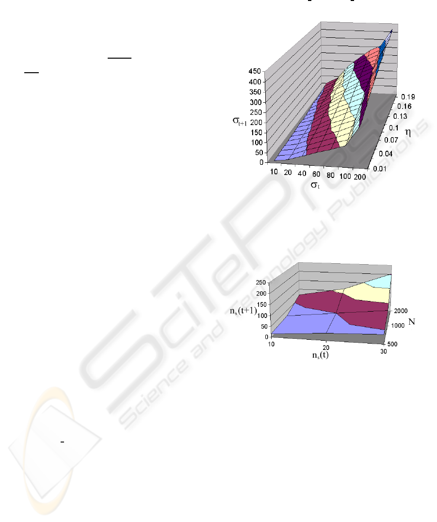
The parametric 3-dimension plots of σ

t+1

f(σ

, ρ, η) are given in Figure (2). This ﬁgure depicts

the case when ρ is constant, and η is the free variable.

Similarly, the 3-dimension plots of σ

t+1

= f(σ

, ρ, η)

when η is constant, and when ρ is the free variable are

given in Figure (3). The general observations that can

be made from these two graphs are: (i) The graphs

are always monotonically increasing; (ii) As the den-

sity increases, even if the CP, η, is maintained con-

stant, the disease will spread; (iii) If the density is

kept constant, the disease will spread (as we see it,

more rapidly) as the CP, η increases; (iv) Since we

are computing Present state/Next State maps, the sat-

uration conditions are never encountered.

Figure 2: The evolution of the ensemble average over 10

experiments of σ

t+1

= f (σ

, ρ, η) as a function of η when

ρ = 0.55 (i.e., when 500 individuals are placed in the 30×

30 grid). The scale for the X and Y axes should be divided

by N = 500.

Figure 3: The evolution of the ensemble average over 10

experiments of n

(t + 1) = f (n

(t), ρ, η) as a function of ρ

when η = 0.05. Observe that the plot here is not of σ, but

rather of n

(·). The value of σ at any point can be obtained

by dividing the value of n

(t+1) by the corresponding value

of N.

3.2 The Testing Phase

The reader will observe that we have reduced our LCP

problem to a Pattern Recognition (PR) or classiﬁca-

tion problem. Indeed, we have transformed the prob-

lem to one of classifying a certain disease outbreak

phenomenon in terms of its contagion parameter, η.

Thus, as in every PR problem, we are ﬁrst required

to do a training phase which trains the classiﬁer, and

then achieve the testing. The question now is one of

devising an efﬁcient testing module which uses the

training graphs and ﬁgures obtained above. We plan

ICAART 2010 - 2nd International Conference on Agents and Artificial Intelligence

to accomplish the Testing by using the SPL as an in-

tegral part of the PR process.

Assume that we currently have η(t), that it is

our current estimate of the true but unknown CP, η

∗

Based on the value of the density of people and the

proportion of sick people within this area, and our cur-

rent understanding of η(t), we can now use our train-

ing plots to locate the current quiescent point on the

corresponding curve. Now, using this as our estimate,

we can determine the proportion of sick people that

would result on the next day, if η

∗

was indeed η(t). If

the number of sick people estimated by η(t) for this

current quiescent point exceeds the actual number of

sick people that do occur, we have an indication that

our current estimate η(t) is too high. In that case, we

chose to decrease η(t) by one step based on the reso-

lution parameter, to obtain η(t + 1). Similarly, if η(t)

underestimates the number of sick people at the next

time instant, η(t + 1) is increased to the next corre-

sponding curve in the testing graphs. As long as these

step-sizes are relatively small and the parameter η

∗

unchanged, the results of Section 3 will guarantee that

η(t) converges to η

∗

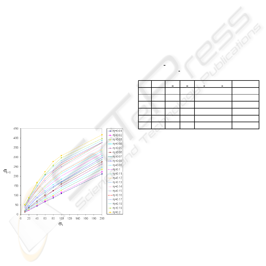
. Of course, to assist us in this

updating, it is more beneﬁcial to have functional plots

of σ

t+1

= f(σ

, ρ, η) as 2-dimensional plots. One of

these plots is given in Figure 4. Similar graphs can

be obtained for the other settings but are not included

here.

Figure 4: The 2-dimensional evolution of the ensemble av-

erage over 10 experiments of n

(t + 1) = f (n

(t), ρ, η) as a

function of η when ρ = 0.55.

A simple example will help clarify matters. Sup-

pose that we are dealing with a value of η

∗

, unknown

to the user, but known to be in the closed interval

[0.01, 0.2]. Also, let us assume that we are deal-

ing with the scenario when N = 500 individuals are

within theW ×W area. We assume that the resolution

parameter R divides [0.0, 0.2] in steps of 0.01. Let

us assume that the current value of η(t) for the test-

ing phase is 0.03. Suppose that the number of sick

individuals at time ‘t’ is n

(t) = 20. If, indeed, η

∗

was 0.03, the number of sick people at time ‘t + 1’

would have been (on the average) n

(t + 1) = 26.

If, however, it turns out that in the testing scenario

(t + 1) = 25, we have an indicator that η(t) under-

estimates η

∗

, and so the solution to the SPL would

dictate that we increase η(t) by the resolution (i.e.,

0.01) to set η(t + 1) to 0.04. The alternate scenario

describes the overestimating case and is omitted. By

successively updating η(t), we move along different

curves on the corresponding 3-dimensional plot de-

scribed by σ

t+1

= f(σ

, ρ, η), to converge to η

∗

Table 1: Results obtained by using the SPL algorithm to

learn the CP when η

∗

= 0.09. The starting value is η(0) =

0.05; the resolution for updating η was set to be 0.01. We

denote by n

s Tr

the number of sick people from the train-

ing phase and by n

s Ts

the number of sick people from the

testing phase.

step η n

s Tr

s Ts

s Tr

< n

s Ts

η± ∆η

0 0.05 10 10

1 0.05 16 20 16<20 yes 0.05+0.01

2 0.06 33 52 33<52 yes 0.06+0.01

3 0.07 90 92 90<92 yes 0.07+0.01

4 0.08 158 169 158<169 yes 0.08+0.01

5 0.09 268 267 268<267 stop η

∗

= 0.09

The parameter learning mechanism described here

was experimentally evaluated to verify the validity of

our analytic results and to examine its rate of con-

vergence. Based on the assumption that the learning

algorithm was ignorant of η

∗

, at any time instant, the

number of sick people was used to update η as de-

scribed earlier. The results of the algorithm are pre-

sented for two cases listed below: (i) In the ﬁrst case,

the value of the unknown η

∗

was set to be 0.09. The

starting value of η was initialized to 0.05. The re-

sults are presented in Table 1, from which we observe

that η(t) converges to η

∗

. (ii) In the second case, the

value of the unknown η

∗

was set to be 0.02. The start-

ing value of η was again initialized to 0.05, and η(t)

again converges to η

∗

(Table 2).

4 CONCLUSIONS

In this paper, we have considered how we can de-

sign a PR system when we have no training sam-

ples. Although such cases are rare, they are ex-

tremely important, for example, when we consider

policy-related decisions concerning the spread of in-

ON USING SIMULATION AND STOCHASTIC LEARNING FOR PATTERN RECOGNITION WHEN TRAINING

DATA IS UNAVAILABLE - The Case of Disease Outbreak

Table 2: Results obtained by using the SPL algorithm to

learn the CP when η

∗

= 0.02. The starting value is η(0) =

0.05; the resolution for updating η was set to be 0.01.

step η n

s Tr

s Ts

s Tr

< n

s Ts

η± ∆η

0 0.05 10 10

1 0.05 16 12 16<12 no 0.05-0.01

2 0.04 18 13 18<13 no 0.04-0.01

3 0.03 19 18 19<18 no 0.03-0.01

4 0.02 27 27 27<27 stop η

∗

= 0.02

fectious diseases. Thus, the PR solution, which in-

volves stochastic learning, considers the problem of

recognizingthe seriousness of a contagion by learning

the Contagion Parameter (CP) in a black box model

involving healthy, sick and contagious individuals. In

our study, PR involves the parameter of interest, η,

which is the probability with which an infected per-

son will transmit the disease to a healthy person. η

is learnt using the theory of Stochastic Point Location

(SPL) which reduces the issue to a PR problem with

Training and Testing phases.

The following are some of the possible avenues

for future work:

1. As mentioned in (Oommen, 1997; Oommen and

Raghunath, 1998; Oommen et al., 2006), apart

from the problem being of importance in its own

right, the SPL also has potential applications in

solving optimization problems. Indeed, a SPL can

be used as a scheme by which the parameters of

an optimization algorithm can be determined, so

as to prevent it from converging all-too sluggishly

on the one hand, or from converging erroneously

or oscillating, on the other. The use of the solution

to the SPL to optimally converge to η

∗

within our

model of contagion is open.

2. An SPL can also be used to assist in the design of

neural networks. Thus, if we consider the back-

propagation neural network, it is well known that

given a particular input, the network uses its “cur-

rent” set of weights to compute the corresponding

output. The obtained output is compared to the

expected output and the network weights are con-

sequently modiﬁed so as to minimize the expected

resultant error. Thus, we could use the solution to

the SPL to devise neural techniques to learn η

∗

3. The problem of learning η

∗

when this quantity

changes with time is an extremely interesting

problem. We believe that solutions to this prob-

lem could have profound implications in a real-

life pandemic.

4. It would be very interesting to see if a SPL solu-

tion can be applied to a contagion model which

is more general than the one we have considered

here. We believe that such a strategy is both fea-

sible and expedient.

REFERENCES

Chin, J. (2000). Control of Communicable Disease Manual.

American Public Health Association, Washington.

Diekmann, O. and Heesterbeek, J. A. P. (2000). Mathe-

matical Epidemiology of Infectious Diseases: Model

Building, Analysis and Interpretation. John Wiley.

Greenland, S. (343–357, 1998). Basic methods for sensitiv-

ity analysis and external adjustment. In K.J. Rothman

KJ and S. Greenland - Modern epidemiology, 2nd ed.

Philadelphia, PA: Lippincott-Raven Publishers. Lip-

pinicot Williams & Wilkins.

Lakshmivarahan, S. (1981). Learning Algorithms Theory

and Applications. Springer-Verlag.

Narendra, K. S. and Thathachar, M. A. L. (1989). Learning

Automata. Prentice-Hall.

Oommen, B. J. (SMC-27B:733–739, 1997). Stochastic

searching on the line and its applications to parameter

learning in nonlinear optimization. In IEEE Transac-

tions on Systems, Man and Cybernetics.

Oommen, B. J., Kim, S. W., Samuel, M., and Granmo,

O. C. (SMC-38B:466-476, 2008.). A solution to the

stochastic point location problem in meta-level non-

stationary environments. In IEEE Transactions on

Systems, Man and Cybernetics.

Oommen, B. J. and Raghunath, G. (SMC-28B:947–954,

1998). Automata learning and intelligent tertiary

searching for stochastic point location. In IEEE Trans-

actions on Systems, Man and Cybernetics.

Oommen, B. J., Raghunath, G., and Kuipers, B. (SMC-

36B:820–836, 2006.). Parameter learning from

stochastic teachers and stochastic compulsive liars. In

IEEE Transactions on Systems, Man and Cybernetics.

Poznyak, A. S. and Najim, K. (1997). Learning Automata

and Stochastic Optimization. Springer-Verlag, Berlin.

Robert, C. P. and Casella, G. (2005). Monte Carlo Statisti-

cal Methods (Springer Texts in Statistics). Springer.

Thathachar, M. A. L. T. and Sastry, P. S. (2003). Net-

works of Learning Automata : Techniques for Online

Stochastic Optimization. Kluwer Academic, Boston.

ICAART 2010 - 2nd International Conference on Agents and Artificial Intelligence