
”RAIN FALL” PARTICLE MODEL FOR SHAPE RECOVERY AND
IMAGE SEGMENTATION
Wen Shi and Shahram Payandeh
Experimental Robotics and Graphics Laboratory, School of Engineering Science, Simon Fraser University
8888 University drive, Burnaby, Canada
Keywords:
Image Segmentation, Shape recovery, SPH (Smoothed particle Hydrodynamics), ”Rain Fall” model.
Abstract:
This paper studies the problem of shape recovery and image segmentation with examples related to medical
imaging. Our purpose is to explore an alternative physics based image segmentation model in comparison with
parametric intensive methods such as active contour or level set approaches. The proposed model can offer a
more computational efficient approach. As an early attempt, a novel segmentation method based on physically
motivated particle system is presented, analyzed and integrated for 2D and 3D applications. Different from
previous particle based segmentation method, our proposed approach is governed physically by fluid dynamic
model. Additionally a novel ”rain fall” model is presented as an alternative paradigm for shape reconstruction
and image segmentation when working with complex 2D and 3D medical images. In this paper, an overview
of fluid mechanical model and fluid particle simulation process is presented as well. Segmentation results on
2D images and shape recovery of 3D images are presented followed by discussions and conclusions.
1 INTRODUCTION
Deformable Models for image segmentation and
shape recovery have been attracting considerable at-
tentions in the past decades (Ajit, 1996) . Classi-
cal methods such as SNAKE (Michael, 1987) have
gained popularity in various aspects of computer vi-
sion, computer graphics and image analysis. Their
main features can be summarized as follows: a) the
methodology is analogous to the way that elastic
physical objects respond to the applied forces in the
physical world, hence the established model is very
natural and intuitive; b) the behaviour of geometrical
shape is constrained by the forces which can be de-
fined based on the features of the image. c) due to
their physically based nature, deformable models can
offer a dynamic simulation framework on which real
time computation can be carried out and adaptively
tuned.
Deformable Particle system based segmentation
approaches are developed as modeling tools of de-
formable model (Andrei C. 2004) (Herng-Hua, 2008).
They are motivated by both deformable image seg-
mentation method and particle based graphical tech-
nique. Here more physical constraints can be incorpo-
rated into the approach, since the external image fea-
ture based forces and the internal smoothing forces
are all modeled as real physical forces ,e.g. electro
static force (Andrei C. 2004) or charged fluid force
(Herng-Hua, 2008) .
This paper presents an early attempt to explore an
alternative solution based on fluid particles for shape
recovery and image segmentation problem. It also
presents results on both 2D image segmentation and
3D shape recovery. The paper is organized as follows:
Section 2 presents an overview of the fluid particle
model and the application to medical image segmen-
tation and shape recovery. Section 3 shows the results
for both 2D and 3D images along with discussions.
Section 4 summarizes the contributions and discusses
the potential benefits and possible extensions in the
future.
2 FLUID PARTICLE MODEL FOR
IMAGE SEGMENTATION
In this paper, we consider the particles to form a fluid
system where the internal forces among particles are
governed by hydrodynamics laws. Based on the im-
age features, the external image forces can be defined
analogously to gravity or viscous forces which would
affect the movements of the particles.
68
Shi W. and Payandeh S. (2010).
”RAIN FALL” PARTICLE MODEL FOR SHAPE RECOVERY AND IMAGE SEGMENTATION.
In Proceedings of the Third International Conference on Bio-inspired Systems and Signal Processing, pages 68-73
DOI: 10.5220/0002712700680073
Copyright
c
SciTePress

2.1 Fluid Particle Hydrodynamics
Fluid Dynamics is governed by continuous differen-
tial equations. For example, (Andrei, 2006) imple-
mented two partial differential equations to describe
the model. In our model, fluid system is discretized
into particles, where a computational tool is needed
in order to calculate the continuous formulations in
a discretized fashion. SPH (Smoothed Particle Hy-
drodynamics) is a computational tool which was first
proposed in astronomy for the simulation of clusters
(Joe J. 1992), and widely used in simulating fluid and
gas models. The main functional of SPH is to ap-
proximate continuous function values and carry out
continuous function calculations such as gradient or
Laplacian on discretized particles or elements. This
can be illustrated by following equations:
< A(x) >=
∑
j
ω
h
(||x −x
j
||)
m
j
ρ
j
A
j
(1)
< ∇A(x) >=
∑
j
∇ω
h
(||x − x
j
||)
m
j
ρ
j
A
j
(2)
< ∆A(x) >=
∑
j
∆ω
h
(||x − x
j
||)
m
j
ρ
j
A
j
(3)
Where the sign <> denotes SPH approximation
(M.H. Everts. 2004). A(x) is a continuous function,
< A(x) > is its SPH approximation on discretized par-
ticles. A
j
is the function value on the j-th particle. x
denotes the current particle of interest, x
j
denotes its
neighbor particle j. m
j
and ρ
j
are the mass and den-
sity of the j-th particle. ω
h
is a weighting kernel func-
tion.
ω(r, h) =
315
64πh
9
r < h,
0 r > h.
(4)
One form of the weighting kernels is described in
equation (4) which is also utilized in this paper. In (4)
r is the distance between particles and h is a pre-set
cut-off distance.
The motion of the fluid particles is governed by
the following equation (Clayton, 1975):
˙v =
f
pressure
ρ
+
f
viscous
ρ
+
f
external
ρ
(5)
Where ρ is density, v is the velocity thus ˙v is the ac-
celeration. force created due to the change in the pres-
sure can be calculated as the negative pressure differ-
ences f
pressure
= −∇P, Here pressure P is computed
as P = k((
ρ
ρ
0
)
γ
− 1), where ρ
0
is the standard density
of the fluid under the standard atmosphere pressure,
k is a constant through which we can modify the in-
compressibility of the fluid, γ is a constant which also
affects the compressibility. Low value of γ models
the fluid particles to be more compressible. The ac-
celeration can be directly computed as
f
pressure
ρ
= − <
∇P
ρ
>, the term
∇P
ρ
can be further calculated as
∇P
ρ
=
∇(
P
ρ
)+
P
ρ
2
∇ρ. Using the above definitions and deriva-
tives we can calculate the acceleration caused by pres-
sure as
f
pressure
(p
i
)
ρ
i
=
∑
j
∇ω
i j
m
j
(
P
j
ρ
2
j
) +
P
i
ρ
2
i
. Where ω
i j
is the weight value between the i-th and j-th parti-
cle, ρ
i
is calculated also using SPH approximation as
ρ
i
=
∑
j
ω
i j
m
j
. Acceleration caused by viscosity ef-
fect is defined as
f
viscous
ρ
= µ∆v , Which is calculated
using SPH approximation as
f
viscous(x
i
)
ρ
i
= µ < ∆v >
i
=
µ
∑
j
∆ω
i j
m
j
ρ
j
(v
j
− v
i
). The motion of the fluid parti-
cles can now be defined by integrating the equation
along the streamline of particles. The fluid simulation
is achieved by applying an integration approximation
(e.g. Euler’s method) to calculate the velocity and po-
sition of each fluid particle (6).
v
i
(t + ∆t) = v
i
(t)+ ˙v
i
∆t,
P
i
(t + ∆t) = P
i
(t)+ v
i
(t)∆t.
(6)
where P
i
(t) is the position of the i-th fluid particle at
the time instance t.
2.2 Application of Fluid Particle to
Image Segmentation
In order to apply fluid particles for image segmenta-
tion, we need to define and incorporate the external
image force f
external
in equation 5. For instance when
dealing with binary images, we can obtain the gra-
dient map of the simple binary image of which the
pixels have the value equal to 255 in the edge region
and 0 in the rest regions. Then we can incorporate the
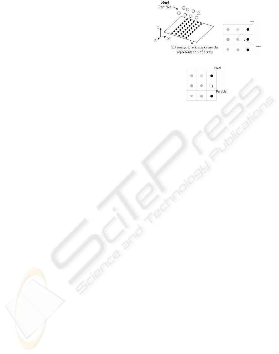
image pixel values to establish an external force field.
Equation 7 models the external image force as pro-
portional to the gradient values and distance between
fluid particles and pixel grids.
f
image
=
∑
N
j
ω(r, h)(P
pixel
j
− P
particle
i
)U
jth−pixel
η
f
external
= f
image−βv
i
(t)
(7)
Where P
particle
i
is the position of the current parti-
cle of interest; P
pixel
j
is the position of the j-th pixel.
U
jth−pixel
is the gradient value of that pixel; η is an ad-
justable coefficient. N is the number of pixels in the
image. −βv
i
(t) is the damping force which consumes
and minimizes the kinetic energy of the ith particle, β
is an adjustable damping coefficient. We apply the lo-
calization weighting function in equation (4) to select
pixels which are closer to the fluid particle of inter-
est within a pre-defined adjustable cut-off radius h.
"RAIN FALL" PARTICLE MODEL FOR SHAPE RECOVERY AND IMAGE SEGMENTATION
69
By applying the image force f
image
in equation (7) to
each fluid particle, the fluid flow would gradually be
attracted to the boundaries of the object in the image
and finally reside along the boundaries.
There are several tunable parameters in the fluid
model(such as the initial velocity of the particles, cut-
off radius of the weighting function and the parame-
ters in calculation of internal fluid forces), which need
to be selected for a particular fluid-flow simulation.
One approach can be to first adjust the parameters of
the fluid particles in the absence of the real image un-
till an initial smooth laminar flow is obtained; then by
defining the initial positions of the fluid particles, we
can accomplish the segmentation. As it will be seen in
our experimental studies, the fluid particles are initial-
ized in the image plane along one side for segmenting
the simple 2D binary image.
2.3 ”Rain Fall” Model
In general, when applying deformable model based
segmentation to 2D images (e.g. classical SNAKE
algorithm), the computation is carried out in the im-
age plane. In this paper, our approach for segment-
ing complex 2D images and recovering 3D shapes is
based on the physical notion of the ”Rain Fall”, where
the fluid particles outside the image plane would drop
down onto the image. Computationally this can be
achieved by initializing the fluid particles outside
the image plane (or the image space for 3D image),
where the fluid particles will ”drop” down onto the
plane/space to do the segmentation. The above notion
and the follow-up segmentation process is analogous
to the phenomenon of rain pouring down to a plane or
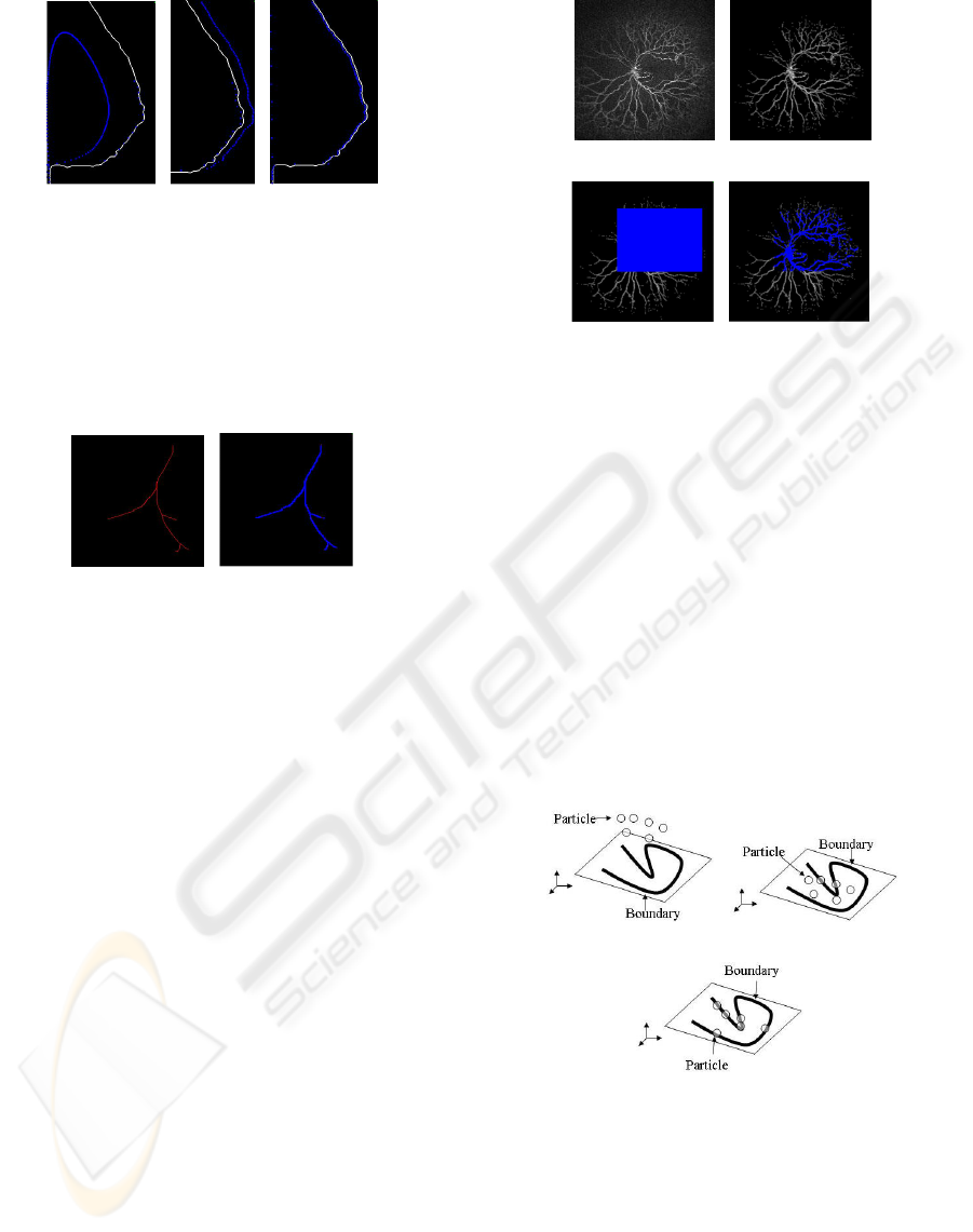
a cavity. Figure 1(a) to 1(c) illustrate the conceptual
model of the ”Rain fall” model. This approach can be
considered as a segmentation method initiated in 3D
space.
When the fluid particles reached the image plane,
they would stop falling and start to flow under the
influence of the image forces as discussed in equa-
tion (6) figure 1(c). This process is analogous to the
natural phenomenon where the rain fall down to the
ground and flow influenced by the terrain topogra-
phy to form some paths. In our approach, the ”ter-
rain topography” are the image features such as object
boundaries.
3 EXPERIMENTAL STUDIES
This section presents initial experimental studies ex-
ploring the method of this paper. The results are pre-
sented in a range from 2D binary image, 2D vessel
(a) (b)
(c)
Figure 1: illustration of ”Rain Fall” model, the black marks
are the pixels in the image, while the white circles repre-
sent the fluid particles. The ”Rain” particles are initialized
outside the image plane. The pixels with darker color rep-
resents larger pixel value. (a) Initial step of ”Rain Fall”,
The particles are initialized outside the image plane; (b)
Snapshot of a single particle when dropping onto the image.
Each particle has been assigned an initial velocity vector
whose direction vertically points down to the image plane;
(c)Snapshot of a single particle when it reaches the image
plane and is attracted by a pixel with larger pixel values.
The particle moved toward the pixel and finally resides on
it.
image to 3D image. In order to demonstrate the seg-
mentation, we show series of results including the ini-
tial stage, intermediate stage and the final stage.
3.1 Results on 2D Images
Figure 2(a) to 2(c) illustrate the segmentation process
of fluid particles toward 2D binary image. For the 2D
binary image, the fluid particles are initialized along
the left side of the image. The constant γ for com-
puting pressure force in equation 5 is set to be 2, the
constant µ for computing viscous force in equation 5
is set to be 7, the cut-off distance h in equation (4)
is set to be twice of the pixel spacing of the target
image. Each fluid particle is assigned an initial ve-
locity of 1 milli-meter per second, so they can start
to move at the beginning. The direction of the initial
velocity vector points to the boundary. Figure 2(a)
shows the fluid particles start to move under the at-
traction of the boundary. Figure 2(b) shows the fluid
particles go through the boundary, this is due to the
remaining kinetic energy. Figure 2(c) shows that fi-
nally the fluid particles reside on the boundary.(i.e.
the boundary acts like a valley toward which the fluid
flows). Figure 3(a) and 3(b) show the result of the
method working on vascular structure 2D image. In
BIOSIGNALS 2010 - International Conference on Bio-inspired Systems and Signal Processing
70
(a) (b) (c)
Figure 2: Segmentation results for 2D binary image. In this
application fluid particles are initialized on the left side of
the image plane (a) Beginning step. Each particle is as-
signed an initial velocity vector whose direction points to
the right boundary. Influenced by the image forces, parti-
cles are attracted toward the boundary; (b) Propagating step,
particles are oscillating around the boundary; (c) Final step,
particles reside along the boundary.
(a) (b)
Figure 3: Segmentation result for 2D vessel image with bi-
furcation. The fluid particles are initialized within the image
plane, (a) Original image; (b) Segmented Image.
order to segment the bifurcation along the path, we
initialize two fluid particles streamlines on both sides
of the image. The parameter setup is the same as the
experiment in figure(2). Since the process steps are
similar to Figure(2), we only show the original image
in Figure 3(a) and the final result in Figure 3(b).
However when dealing with 2D image with complex
vascular structures and background noise, the simple
streamlines initialization is not sufficient. For exam-
ple if there are many bifurcations along each vascular
structure in the vessel image and particles are only
initialized within the image plane, they will be only
attracted by outer vascular structures and fail to seg-
ment the inner vessels. As a result we implement
our proposed ”Rain fall” model. Figure 4(a) to 4(d)
demonstrate the results on 2D image with complex
vessel structures. Figure 4(a) is the original image. In
this application, Thresholdfilter is applied to take out
some of the background noise in the original image.
The image after thresholding is shown in figure 4(b).
The fluid particle parameters which are used in this
experiment are similar to the above 2D experiments,
however we initialize the fluid particles such that the
initial positions of them are set to be on top of the im-
age and they are arranged evenly distributed (during
the rain fall, the rain particles are assumed to be dis-
(a) (b)
(c) (d)
Figure 4: Segmentation result for 2D complex vessel image.
The ”Rain Fall” model is implemented, (a) Original 2D ves-
sel image; (b) Thresholded 2D vessel image; (c) Initialized
Particles. Particles are arranged to be evenly distributed,
which form a square array on top of the image. The spacing
of the particles are twice of the image pixels(thus the parti-
cles are too close to be recognized); (d) Segmented Image.
tributed evenly). The direction of the initial velocity
vector is set to point toward the image plane. When
the segmentation starts, the fluid particles will move
toward the image or ”drop” down to the image. We
assign each particle an equal initial velocity which is
1 milli-meter per second to start the simulation. If the
particles hit the image plane like ”rain fall”, they will
stop falling and move under the influence of the fluid
mechanics and the attraction of the image forces.
(a) (b)
(c)
Figure 5: Conceptual diagram for the ”Rain Fall” model,
(a)Initialization stage of ”Rain Fall” model;(b) Segmenta-
tion stage1 (Particles reach the image plane) of ”Rain Fall”
model; (c) Segmentation stage2 (Particles are attracted by
the boundary in the image) of ”Rain Fall” model.
Figure 5(a) to 5(c) explains the concept idea. In
the practical application we initialize the fluid parti-
cles so that they are placed in another 2D plane just
on top of the image, as shown in figure 4(c). We can
"RAIN FALL" PARTICLE MODEL FOR SHAPE RECOVERY AND IMAGE SEGMENTATION
71
obtain the final segmented image, as illustrated in fig-
ure 4(d).
3.2 3D Shape Recovery
Since the fluid particles in ”Rain Fall” model are
falling from the outside of the 2D image plane, they
have 3 degrees of freedom of motion when compared
with the standard 2D particle based models. As a re-
sult, it is possible to take advantage of this feature
and extend the model to work on the 3D image data.
Analogous to the extraction of boundaries in 2D im-
age, in 3D image we can establish the external image
forces by calculating the spatial gradient of the vox-
els(volume pixel), then substitute the magnitude of
the spatial gradient of each voxel for the pixel gradi-
ent value U
jth−pixel
in equation 7. Since voxels which
have large magnitude of spatial gradient are the ones
lying on the surface of the object in the image, when
the fluid particles drop toward the object, they will be
attracted by the surface voxels, as a result the object
shape can be recovered by the fluid particles. Follow-
ing this idea, an application of ”Rain Fall” model on
shape recovery of 3D image is developed.
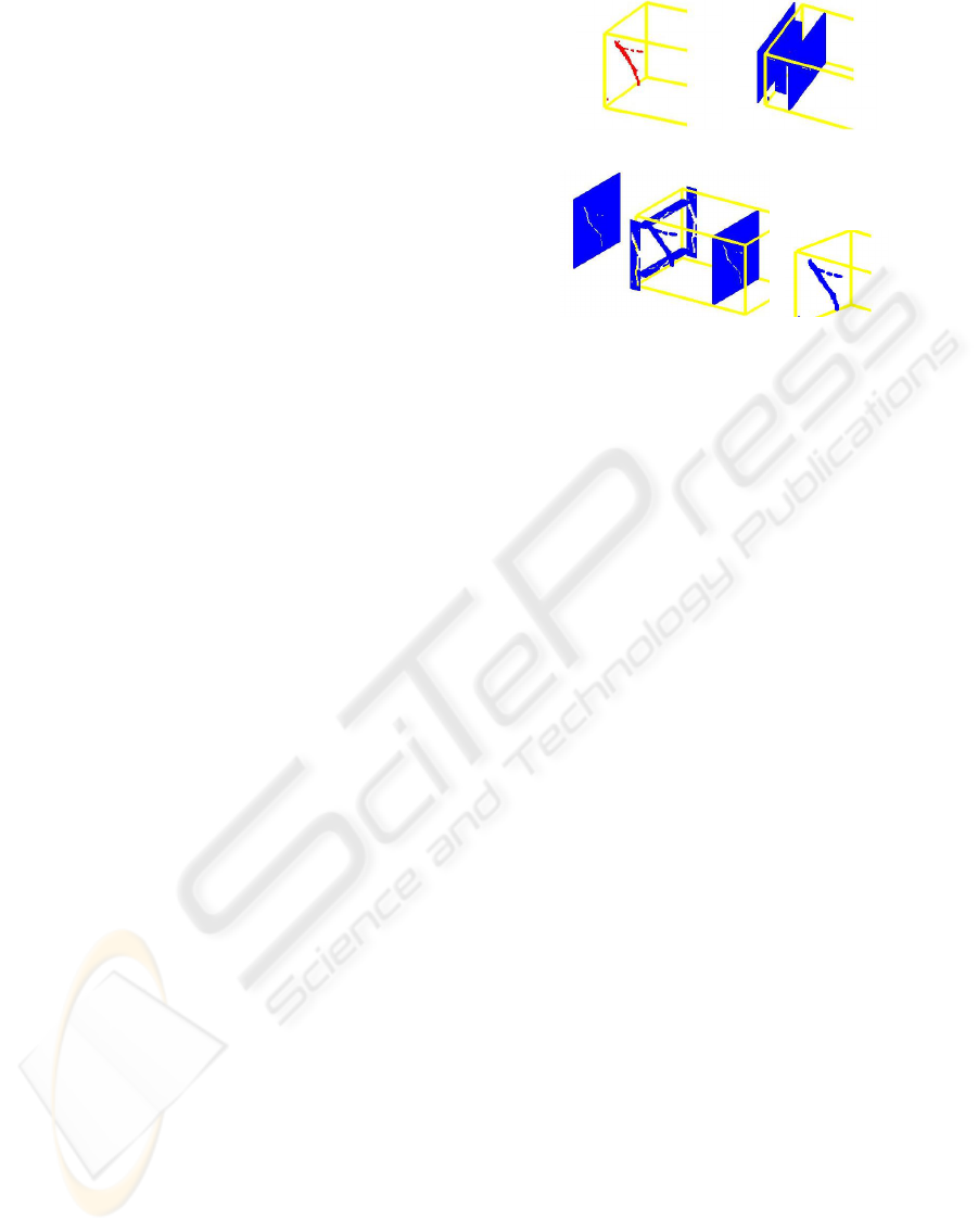
Figure 6(a) to Figure 6(d) illustrate the results.
Figure 6(a) is the original 3D vascular structure data
obtained by MRI, which is visualized using OpenGL
graphic rendering engine. In order to carry out the
shape recovery, we need to initialize the fluid parti-
cles properly so that the entire 3D object can be inside
the motion range of the particles. Analogously to the
initialization of ”Rain Fall” model on segmenting 2D
images, We can initialize The fluid particles to stay
within other planes. However since the target now is
a 3D object, we initialize the particles such that they
form the 6 boundary planes of a bounding cubic space
where the 3D object is located figure 6(b). Thus the
target object is entirely covered by the particles. Then
each particle is assigned an initial velocity vector hav-
ing the same magnitude and the direction pointing
vertically toward the target 3D object. Other param-
eter settings are similar to 2D application. When the
”Rain Fall” simulation starts, some of the fluid par-
ticles are attracted by the image forces generated by
the surface voxels of the image object and move to-
ward the surface. When some of the particles reach
the surface, they will eventually stop moving and stay
on the surface, others will keep moving and eventu-
ally fall outside the cubic space. This is illustrated in
figure 6(c). The final recovery result is displayed in
figure 6(d).
(a) (b)
(c) (d)
Figure 6: 3D shape recovery, (a) Original 3D vessel im-
age with the bounding volume; (b) Initialized Particle plains
(The particle plains are the bounding plane of the bounding
volume). The particles start to move; (c) after fluid flow.
Some particles are attracted by and move toward the surface
voxels, finally they reside on the surface; (d) Recovered 3D
Shape.
3.3 Discussion
Several novel features of the fluid particles ”Rain
Fall” model are worth to mention. One is the ability
to segment complex structures in 2D images. Tradi-
tional deformable model such as SNAKE (Ajit, 1996)
and electric particles method (Herng-Hua, 2008) can
only deal with convex or simple concave object in 2D
image, since these methods only work inside the im-
age plane. For the ”rain fall” model, the fluid parti-
cles are initialized outside the image plane and ”fall”
down to the plane to do the segmentation, thus it has
more degrees of freedom and can be applied to seg-
ment complex 2D images such as vascular images.
Another feature is the ability to recover 3D shapes.
Since particles can move in 3D space, they also can
be attracted by some external force field within certain
range of space. As a result, when being attracted by
the surface voxels of 3D object, the ”Rain Fall” parti-
cles recover the 3D shape. However the current ”Rain
Fall” model is still sensitive to background noise and
the segmentation result can be affected. For example
in figure 4(d), we can see that there are some uncon-
nected particles inside the vascular structures. This is
due to the corruption of the vascular pixels by noise.
As an example to deal with the problem, we im-
plement k-nearest neighbourhood checking to double
check the pixel labels. This is illustrated in figure 7(a)
where the ith pixel is corrupted by the noise. After
checking its 8-nearest neighbourhood pixels, there are
more than 2 pixels belonging to the vascular structure,
illustrated as Neighbour pixel 1 and 2. In this case
BIOSIGNALS 2010 - International Conference on Bio-inspired Systems and Signal Processing
72
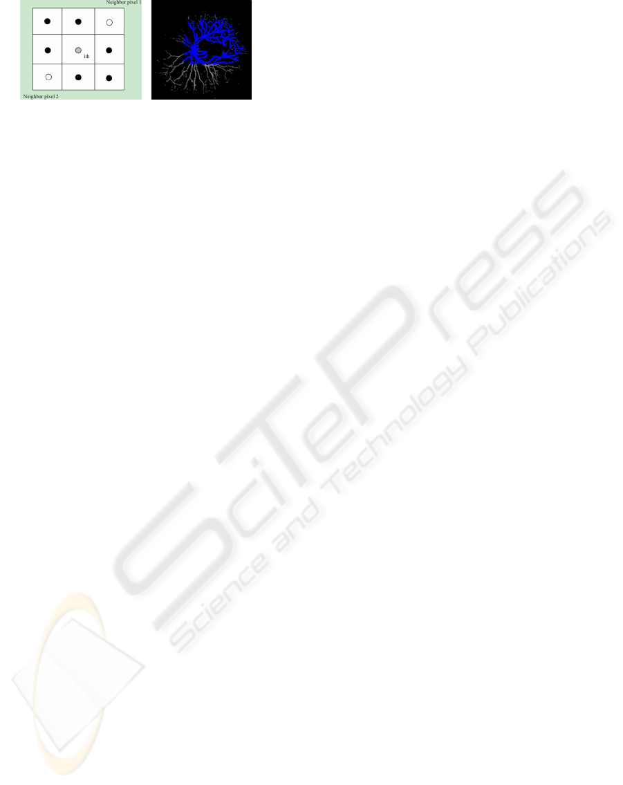
(a) (b)
Figure 7: 8-nearest neighborhood checking, (a) Concept di-
agram; (b) After neighborhood checking.
the ith pixel should be labeled as vascular pixel. The
resulting image is shown in figure 7(b). Compared
with figure 4(d), the vascular structure has less uncon-
nected regions in the vascular structures.Apparently
other anti-noise post-processing methods can be im-
plemented as well.
4 CONCLUSIONS AND FUTURE
WORK
In this paper, we recreate a fluid particle based image
segmentation and shape recovery method which be-
longs to the deformable model category particularly
the particle based deformable model. Different from
the existing particle based method, we applied fluid
mechanical model through using SPH (Smoothed Par-
ticle Hydrodynamics) to compute the internal con-
straining forces among particles. Upon minimizing
the kinetic energy of the fluid particle system in terms
of the internal fluid forces and the external image
forces, image segmentation can be achieved. In order
to complete the image segmentation, we explored the
initialization of the fluid particles and developed the
”Rain fall” model as to segment complex structures
in the image. Finally we tried to segment the compli-
cated vessel image. Upon using threshold filter as the
pre-processor and 8-nearest neighbourhood checking
as the post-processor, the segmented vessel image is
good in connectivity and smoothness. Finally we ex-
tended the ”Rain Fall” model to recover 3D object
shape. As pointed out in the paper, our method can
have a better potential for segmenting complex struc-
tures such as non convex vascular structure compared
with the existing methods due to the higher degrees of
motion freedom of the particles. We also extend our
work to 3D shape recovery. More advanced anti-noise
pre-processing methods are required such as vessel-
ness diffusion enhancement filter (Rashindra, 2006)
in the future study. We can collect voxels inside the
volume of the segmented object as oppose to only the
boundaries, which can be used in the point-based ren-
dering of deformable objects in our VR(Virtual Real-
ity) training project.
REFERENCES
Ajit Singh, Dmitry Goldgof, Demetri Terzopoulos. (1996).
Deformable models in Medical image Analysis. In
Medical image analysis 1996. Elsevier Science Press.
Michael Kass, Andrew Witkin, Demetri Terzopoulos.
(1987). Snake: Active Contour Models. In Interna-
tioanl journal of Computer Vision, 321-331. Kluwer
Academic Publishers.
Andrei C. Jalba, Michael H.F. Wilkinson, Jos B.T.M.
Roerdink. (2004). CPM: A Deformable Model for
Shape Recoveryand Segmentation Based on Charged
Particles. In IEEE Transactions on Pattern Analysis
and Machine Intelligence, Vol. 26, No. 10, October
2004. IEEE Computer Society.
Herng-Hua Chang and Daniel J. Valentino. (2008). An
Electrostatic Deformable Model for Medical Image
Segmentation. In Comput Med Imaging Graph. 2008
January ; 32(1): 2235..
Andrei C. Jalba and Jos b.T.M. Roerdink. (2006). A
Physically-Motivated Deformable Model Based on
Fluid Dynamics In ECCV 2006, Part 1, LNCS 3951,
pp. 496-507,2006 Springer-Verlag Berlin Heidelberg
Rashindra Manniesing, Max A. Viergever, Wiro J. Niessen.
(2006). Vessel enhancing diffusion A scale space rep-
resentation of vessel structures. In Medical Image
Analysis 10 (2006) 815-825. Elsevier Science
Joe J. Monaghan. (1992). Smoothed Particle hydrodynam-
ics. In Annu. Rev. Astron. Physics, 30:543, 1992.
Joe J. Monaghan. (2005). Smoothed Particle hydrodynam-
ics. In Reports on progress in Physics, 68:1703-
1759,2005.
M. Mller, R. Keiser, A. Nealen, M. Pauly, M. Gross and
M. Alexa. (2004). Point Based Animation of Elas-
tic, Plastic and Melting Objects. In Eurograph-
ics/ACM SIGGRAPH Symposium on Computer Ani-
mation (2004) Eurographics Association
M.H. Everts H. Bekker A.C. Jalba J.B.T.M. Roerdink.
(2006). Particle Based Image Segmentation with Sim-
ulated Annealing.
T. Deschamps, P. Schwartz, D. Trebotich, P. Colella, D. Sa-
loner, R. Malladi. (2004). Vessel segmentation and
blood flow simulation using Level-Sets and Embed-
ded Boundary methods. In International Congress Se-
ries 1268 (2004) 75 80 Elsevier Science
Clayton T. Crowe, John A. Roberson. (1975). Engineering
Fluid Mechanics. Houghton Mifflin Co,, 1975
"RAIN FALL" PARTICLE MODEL FOR SHAPE RECOVERY AND IMAGE SEGMENTATION
73
