FINDING DISTANCE-BASED OUTLIERS IN SUBSPACES
THROUGH BOTH POSITIVE AND NEGATIVE EXAMPLES
Fabio Fassetti and Fabrizio Angiulli
DEIS, University of Calabria, Italy
Keywords:
Data mining, Example-based outlier detection, Genetic algorithms.
Abstract:
In this work an example-based outlier detection method exploiting both positive (that is, outlier) and negative
(that is, inlier) examples in order to guide the search for anomalies in an unlabelled data set, is introduced.
The key idea of the method is to find the subspace where positive examples mostly exhibit their outlierness
while at the same time negative examples mostly exhibit their inlierness. The degree to which an example
is an outlier is measured by means of well-known unsupervised outlier scores evaluated on the collection of
unlabelled data.
A subspace discovery algorithm is designed, which searches for the most discriminating subspace. Experi-
mental results show that the method is able to detect a near optimal solution, and that the method is promising
from the point of view of the knowledge mined.
1 INTRODUCTION
Unsupervised outlier detection techniques search for
the objects most deviating from the data population
they belong to. These techniques are employed on
unlabelled data sets, that is when no a priori infor-
mation about what should be considered normal and
what should be considered exceptional is available,
and outliers are singled out on the basis of certain out-
lier scores that can be assigned to each single object.
However, in addition to the unlabelled data set,
very often also examples of normality and examples
of abnormality are available. In this scenario it is then
of interest to modify the mining technique in order to
take advantage of these examples.
In this work an example-based outlier detection
method exploiting both positive (that is, outlier) and
negative (that is, inlier) examples in order to guide
the search for anomalies in an unlabelled data set,
is introduced. The task here introduced is novel, in
that previous methods are able to exploit only posi-
tive examples. The key idea of the method is to find
the subspace where positive examples mostly exhibit
their outlierness while at the same time negative ex-
amples mostly exhibit their inlierness.
The method can be useful when a small amount of
labelled data is available, e.g. a few patients for which
an ascertained diagnosis is known, and the individuals
to be single out are anomalous, that is their occurrence
frequency is very low, e.g. consider people affected
by a rare disease.
The degree to which an example is an outlier is
measured by means of well-known unsupervised out-
lier scores evaluated on the collection of unlabelled
data. A distance-based unsupervised outlier scores is
employed, that is the mean distance of the object from
its k nearest neighbors (Angiulli and Pizzuti, 2002).
A subspace is then deemed to comply with the pro-
vided examples if a separation criterium between out-
lier scores associated with positive examples and out-
lier scores associated with negative examples is sat-
isfied, and, moreover, the difference between the for-
mer and the latter ones is positive.
The most discriminating subspace is that which
maximizes the above difference. Note that this mea-
sure is not monotonic with respect to subspace con-
tainment. While from a semantic point of view this
property can be considered a desideratum, from the
algorithmic point of view the above property makes
very difficult to guide search towards the right sub-
space.
A subspace discovery algorithm is designed,
which searches for the most discriminating sub-
space. As already noted, finding this subspace is a
formidable problem due to the huge search space,
while the non-monotonicity of the measure to op-
5
Fassetti F. and Angiulli F. (2010).
FINDING DISTANCE-BASED OUTLIERS IN SUBSPACES THROUGH BOTH POSITIVE AND NEGATIVE EXAMPLES.
In Proceedings of the 2nd International Conference on Agents and Artificial Intelligence - Artificial Intelligence, pages 5-10
DOI: 10.5220/0002699600050010
Copyright
c
 SciTePress

timize makes difficult to alleviate the cost of the
search. The introduced mining technique is based on
the paradigm of genetic algorithms, which are able to
provide good approximate solutions to the problem of
optimizing a multidimensional objective function.
The rest of the work is organized as follows. In the
rest of this section, work related to the one here pre-
sented is briefly surveyed and major differences are
pointed out. In Section 2, the novel task tackled with
in this work is formally defined. Subsequent Section
3 presents the ExampleBasedOutlierDetection algo-
rithm. Section 4 describes experiments on both syn-
thetic and real data sets. Finally, Section 5 draws con-
clusions and future work.
1.1 Related Work
Next some outlier detection methods working on
subspaces and/or exploiting examples are briefly re-
called. Contributions of this work are clarified by
pointing out differences with related methods while
discussing them.
The work (Aggarwal and Yu, 2001) detects
anomalies searching for subspaces in which the data
density is exceptionally lower than the mean den-
sity of the whole data. Promising subspaces are de-
tected by employing a technique based on genetic al-
gorithms. Although this method works on the sub-
spaces, it does not contemplate the presence of exam-
ples.
In (Zhang and Wang, 2006) the interest is on
searching for the subspaces in which the sum of the
distances between a fixed object and its nearest neigh-
bors exceeds a given threshold. A dynamic subspace
search exploiting sampling is presented and compared
with top-down and bottom-up like techniques. This
work exploits only one positive example and it has no
negative ones. Furthermore, subspaces in which the
example is exceptional are searched for, while discov-
ery of additional outliers is not accomplished.
The work (Wei et al., 2003) focuses on discover-
ing sets of categorical attributes, called common at-
tributes, being able to single out a portion of the data
base in which the value assumed by an object on a sin-
gle additional attribute, called exceptional attribute,
becomes infrequent with respect to the mean of the
frequencies of the values assumed by the same at-
tribute. Common attributes are determined by select-
ing the sets of frequent attributes of the data base.
In (Zhu et al., 2005) the Outlier by Example
method is introduced. Given a data set and user-
provided outlier examples, the goal of the method
is to find the other objects of the data set exhibiting
the same kind of exceptionality. Data set objects are
mapped into the MDEF feature space (Papadimitriou
et al., 2003), and both user-provided examples and
outstanding outliers, i.e. those that can be regarded
as outliers at some granularity level, are collected to
form the positive training data. Then the SVM algo-
rithm is employed in order to build a classifier sepa-
rating the normal data from the positive training data.
This technique employs only positive examples, is
based on the MDEF measure, and does not work on
subspaces, but instead searches for anomalies in the
full feature space.
In (Zhu et al., 2005), given an input set of exam-
ple outliers, i.e. of objects known to be outliers, the
authors search for the objects of the data set which
mostly exhibit the same exceptional characteristics.
In order to single out these objects, they search for
the subspace maximizing the average value of sparsity
coefficients, that is the measure introduced in (Aggar-
wal and Yu, 2001), of cubes containing user exam-
ples. This method is suited only for numerical at-
tributes, it is based on the notion of sparsity coeffi-
cient, which is different from the notion of distance-
based score, and it can take advantage only of pos-
itive examples, while negative ones are not consid-
ered. Moreover, it must be noted that the sparsity co-
efficient is biased towards small subspaces. Indeed,
in order to prefer larger ones it should take place that
the number of objects is exponentially related to the
number of attributes, a very unlikely situation.
2 PROBLEM STATEMENT
First some preliminary definitions are provided, and
then the example-based outlier score is introduced.
A feature is an identifier with an associated do-
main. A space F is a set of features. An object of
the space F is a mapping among features A ∈ F and
values in the domain of A. The value of the object o
on the feature A ∈ F is denoted by o
A
. A subspace S
of F is any subset of F. The projection of the object
o in the subspace S, denoted by o
S
, is an object of the
space S such that o
S
A
= o
A
, for each A ∈ S. Note that
o
F
= o. The projection of a set of objects O in the
subspace S, denoted by O
S
, is {o
S
| o ∈ O}.
A distance dist on the space F is a semimetric
defined on each pair of objects of each subspace of
F, that is a real-valued function which satisfies the
non-negativity, identity of indiscernibles and symme-
try axioms.
Let a set of objects DS of the space F, called data
set in the following, be available. Let K ≥ 1 be an
integer. The K-th nearest neighbor of o
S
(in the data
set DS), denoted by nn
K
(o
S
), is the object p of DS
ICAART 2010 - 2nd International Conference on Agents and Artificial Intelligence
6

such that there exist exactly K − 1 objects q of DS
with dist(o
S
, q
S
) ≤ dist(o
S
, p
S
).
Outlier Score. In this work, we employ a well-
established distance-based measures of outlierness,
also said outlier score in the following.
The outlier score os(o) of o is defined as follows
(Angiulli and Pizzuti, 2002):
os(o) =
1
K
K
∑
i=1
dist(o, nn
i
(o)).
The outlier score is given by the sum of the distances
between o and its K nearest neighbors in the data set.
Its value provides an estimate of the data set density in
the neighborhood of the object o. The objects o scor-
ing the greatest values of outlier score os(o) are also
called outliers, since they be considered anomalous
with respect to the population under consideration.
Let E be a set of objects. The outlier score sc(E)
of E is defined as the mean of the outlier scores asso-
ciated with the elements of E:
sc(E) =
1
|E|
∑
e∈E
os(e).
Subspace Score. Assume a set O of outlier exam-
ples (or positive examples) and a set I of inlier exam-
ples (or negative examples) are available.
We are interested in finding subspaces where the
outlier examples deviate from the data set population,
the inlier examples comply with the data set popu-
lation, and the separation between these examples is
large.
In order to formalize the above intuition, the fol-
lowing definition of consistent (with respect to a set of
positive and negative examples) subspace is needed.
We say that a subspace S is ρ-consistent, or simply
consistent, where ρ ∈ [0, 1] is a user-provided param-
eter, with respect to a set O of positive examples and a
set I of negative examples, if the ρ percent of the ob-
jects in O
S
, that are the positive examples O projected
in the subspace S, is globally more outlying than the
set of objects in I
S
, that are the negative examples I
projected in the subspace S, while the remaining 1− ρ
percent of the objects in O
S
is individually more out-
lying than all the objects in I
S
, that is to say,
1. sc(O
S
b
) > sc(I
S
), where O
b
is the set of the ⌈ρ|O|⌉
objects o of O having the smallest outlier scores
os(o
S
), and
2. os(o
S
) > max
i∈I
os(i
S
), for each o ∈ (O− O
b
).
where the first condition does not apply if ρ = 0 or O
b
is empty, and, dually, the second condition does not
apply if ρ = 1 or O− O
b
is empty.
In order to measure the relevance of the subspace
S with respect to the above criterium, next the concept
of subspace score is introduced. The subspace score
ss(S) of the space S with respect to set of positive ex-
amples O and set of negative examples I is
ss(S) =

sc(O
S
) − sc(I
S
) , if S is ρ-consistent w.r.t. O and I
0 , otherwise
Note that for a consistent subspace S, the correspond-
ing subspace score ss(S) is always positive.
Moreover, it is worth to point out that the subspace
score is not monotonic with respect to subspace con-
tainment.
Outliers by Example Problem. We are now in the
position of defining the main task we are interested in.
Given an integer n ≥ 1, and a subspace S, the top-
n outliers of DS in S are the n objects o of DS with
maximum value of outlier score os(o
S
).
The outlying subspace S
ss
is defined as
argmax
S
ss(S).
Given a data set DS, a set of positive examples O, a set
of negative examples I, and a positive integer number
n, the Distance-Based Outlier Detection by Example
Problem is defined as follows: find the top-n outliers
in the outlying subspace S
ss
.
3 ALGORITHM
Finding the outlying subspace is in general a
formidable problem. We decided to face it by exploit-
ing the paradigm of genetic algorithms (Holland et al.,
1986; Holland, 1992), a methodology also pursued by
other subspace finding methods for outlier detection
(Aggarwal and Yu, 2001; Zhu et al., 2005). Genetic
algorithms are based on the theory of evolution and
they are probabilistic optimization methods based on
the principles of evolution. These algorithms have
been successfully applied to different optimization
tasks. In the optimization of non-differentiable or
even discontinuous functions and discrete optimiza-
tion they outperform traditional methods since deriva-
tives provide misleading information to conventional
optimization methods.
Genetic algorithms maintain a population of po-
tential solutions. In our context, a potential solution
is a subspace and it is encoded by means of a binary
string, also said a chromosome, of length |F|. The ith
bit of the binary string being 1 (0, resp.) means that
the ith feature of F is (is not, resp.) in the subspace
encoded by the chromosome. At each iteration a fit-
ness value is associated with each chromosome, rep-
resenting a measure of the goodness of the potential
FINDING DISTANCE-BASED OUTLIERS IN SUBSPACES THROUGH BOTH POSITIVE AND NEGATIVE
EXAMPLES
7

Algorithm ExampleBasedOutlierDetection
Input: data set DS on the set of features F, set O of positive examples, set I of negative examples, number K of
nearest neighbors to consider, number n of top outliers to return, parameter ρ
Output: the example-based outliers of DS
1. Let P the initial population of subspaces having size M, obtained by selecting at random M subsets of the
overall set of features F
2. While the convergence criterion is not meet do
(a) For each subspace S in P, determine if S is already stored in the hash table SSTable and, in the positive
case, retrieve its fitness value
(b) Let P
new
= {S
1
, . . . , S
m
} be the subset of P composed of the subspaces which are not stored in SSTable
(c) For each negative example i in I = {i
1
, . . . , i
N
I
}, determine simultaneously the outlier scores
{os(i
S
1
), . . . , os(i
S
m
)}
(d) Let B denote the number ⌈ρ|O| ⌉, and let α
1
, . . . , α
m
(β
1
, . . . , β
m
, resp.) denote the maximum (mean,
resp.) outlier scores associated with the negative examples in the subspaces S
1
, . . . , S
m
, respectively, that
is α
j
= max
i∈I
os(i
S
j
) (β
j
= sc(I
S
j
), resp.), for j = 1, . . . , m
(e) For each positive example o
k
in O = {o
1
, . . . , o
N
O
} do
i. Determine simultaneously the outlier scores {os(o
S
k
) | S ∈ P
new
}
ii. For each subspace S
j
in P
new
do
A. Let O
k, j
be the set composed of precisely the B objects o of {o
1
, . . . , o
k
} having the smallest outlier
scores os(o
S
j
), and let o
k, j
be the object having the (B+ 1)–th smallest outlier score os(o
k, j
S
j
)
B. If either (1) α
j
≥ os(o
k, j
S
j
) or (2) β
j
≥ sc(O
S
j
k, j
), then set P
new
= P
new
− {P
j
}, and set the fitness of the
subspace P
j
to zero and store it in the hash table SSTable
(f) For each subspace S remained in P
new
, compute its fitness as sc(O
S
) − s(I
S
) and store it in the hash table
SSTable
(g) From the set P, select M pairs hS
1
1
, S
2
1
i, . . . hS
1
M
, S
2
M
i of parent subspaces for the next generation (selection
step)
(h) Compute the set of subspaces P
next
= {S
′
1
, . . . , S
′
M
}, where each subspace S
′
j
is obtained by crossover of
the parent subspaces S
1
j
and S
2
j
, for i = 1, . . . , M (crossover step)
(i) Mutate some of the subspaces in the set P
next
(mutation step)
(j) Set the current population P to the next generation P
next
3. Select the subspace S
ss
in P scoring the maximum fitness value
4. Determine the top-n outliers in the subspace S
ss
and return them as the set of the example-based outliers
Figure 1: The ExampleBasedOutlierDetection algorithm.
solution. The current population is iteratively updated
by means of the selection, crossover, and mutation
mechanisms till a convergence is meet. Selection is a
mechanism for selecting chromosomes for reproduc-
tion according to their fitness. Crossover denotes a
method of merging the genetic information of two in-
dividuals; if the coding is chosen properly, two good
parents produce good children. In genetic algorithms,
mutation can be realized as a random deformation of
the strings with a certain probability. The positive ef-
fect is preservation of genetic diversity and, as an ef-
fect, that local maxima can be avoided.
Figure 1 shows the algorithm ExampleBasedOut-
lierDetection which solves the Outliers by Example
Problem. We employed the subspace score as fitness
function for the genetic algorithm. Since computing
the subspace score is expensive, some optimizations
are accomplished in order to practically alleviate its
cost, which are explained next.
First of all, an hash table SSTable of size T main-
tains the latest T subspaces visited by the algorithm,
together with their fitness, and with a timestamp
which is exploited to implement the insertion policy.
This table is used as follows. Before computing the
fitness associated to a subspace, it is searched for in
the hash table. If the subspace is found, then its times-
tamp is updated and then the fitness stored in the table
is employed. Vice versa, when a novel subspace has
to be stored in the hash table, but no more space is
available in the selected entry, the timestamps are ex-
ploited in order to determine the subspace (that is, the
oldest one) that will be replaced with the latest sub-
space.
In this work we employed the Euclidean distance
as distance function. Let S
1
, . . . , S
m
the subspaces of
the current population which are not already stored
ICAART 2010 - 2nd International Conference on Agents and Artificial Intelligence
8

in SSTable. In order to save distance computations,
the outlier scores os(e
S
1
), . . ., os(e
S
m
) associated with
a positive or negative example e are computed si-
multaneously as follows: first the set U is computed
as S
1
∪ . .. ∪ S
m
and, for each A ∈ U, the values
d
A
= (x
A
− y
A
)
2
are obtained, and then the distances
dist(x
S
j
, y
S
j
) are computed as
q
∑
A∈S
j
d
A
.
As a further optimization, the outlier scores as-
sociated with the negative examples are computed
first (see steps 2(c) and 2(d)). Then, while comput-
ing outlier scores associated with positive examples
(see step 2(e)), the outlier scores of the negative ones
are immediately exploited in order to filter out sub-
spaces which are not ρ-consistent (see step 2(e)ii)
and, hence, avoiding useless distance computations.
As selection-crossover-mutation strategies we
used proportional selection, one-point crossover, and
mutation by inversion of a single bit, while as conver-
gence criterion was used an a-priori fixed number of
iterations, also said generations (Holland, 1992).
As far as the temporal complexity of the algorithm
is concerned, say N the number of data set objects,
N
E
the total number of examples, d the number of
features in the space F, and g the number of gener-
ations. In the worst case, for each generation in or-
der to determine outlier scores the distances among
all the examples and all the data set objects are com-
puted, with a total cost O(g∗ N
E
∗ N ∗ d). After hav-
ing determined the outlying subspace S
ss
, in order to
compute the top-n outliers in that subspace, all the
pairwise distances among data set objects are to be
computed, and, then, the top-n outliers are to be sin-
gled out, with a total cost O(N
2
∗ d). Summarizing,
the temporal cost of the algorithm ExampleBasedOut-
lierDetection is O(g∗ N
E
∗ N ∗ d + N
2
∗ d).
4 EXPERIMENTAL RESULTS
In the experiments reported in the following, if not
otherwise specified, the crossover probability was set
to 0.9 and the mutation probability was set to 0.01.
Moreover, the parameter ρ, determining the “degree”
of consistency of the subspace, was set to 0.1.
First of all, we tested the ability of the algorithm
to compute the optimal solution (that is the outlying
subspace). With this aim, we considered a family of
synthetic data sets, called Synth in the following.
Each data set of the family is characterized by the
size D of its feature space. Each data set consists of
1,000 real dimensional vectors in the D-dimensional
Euclidean space, and is associated with about D posi-
tive examples and D negative examples. Examples are
placed so that the outlying subspace coincides with
a randomly selected subspace having dimensionality
⌈
D
5
⌉.
We varied the dimensionality D from 10 to 20 and
run our algorithm three times on each data set. We
recall that the size of the search space exponentially
increases with the number of dimensions D. We set
the population size to 50 and the number of genera-
tions to 50 in all the experiments. The parameter K
was set to 10.
Table 1 reports the results of these experiments.
Interestingly, the algorithm always found the optimal
solution in at least one of the runs. Up to 15 dimen-
sions it always terminated with the right outlying sub-
space. For higher dimensions it reported also some
different subspaces, but in all cases the solution re-
turned is a suboptimal one. Indeed, the second and
third solutions concerning the data set Synth18D are
subsets of the optimal solution both having only a sin-
gle missing feature, while the second solution con-
cerning the data set Synth20D is a superset of the op-
timal one having two extra features. By these exper-
iments it is clear that the method is able to return the
optimal solution or a suboptimal one.
The subsequent experiment was designed to val-
idate the quality of the solution returned by the pro-
posed method. In this experiment we considered the
Wisconsin Diagnostic Breast Cancer data set from the
UCI Machine Learning Repository. This data set is
composed of 569 instances, each consisting in 30 real-
valued attributes, grouped in two classes, that are be-
nign (357 instances) and malignant (212 instances).
The thirty attributes represent mean, standard error,
and largest value associated with the following ten
cell nucleus features: radius, texture, perimeter, area,
smoothness, compactness, concavity, concave points,
symmetry, and fractal dimension.
We normalized the values of each attribute in the
range [0, 1]. Moreover, we randomly selected ten be-
nign instances as the set of negative examples I
wdbc
and twenty malignant instances as the set of posi-
tive examples O
wbdc
. Moreover, we built a data set
DS
wdbc
of 357 objects by merging together all the re-
maining benign instances (that are 347) with other
ten randomly selected malignant examples, say them
DS
O
wdbc
.
We set the number of neighbors K to 50, and the
number of top outliers n to 20. First of all, we com-
puted the distance-based outliers in the full feature
space. We found that among the top twenty outliers,
six of them belong to the set DS
O
wdbc
(corresponding to
the 60% of DS
O
wdbc
). Next, we run the ExampleBased-
OutlierDetection algorithm. The outlying subspace
S
ss
wdbc
found was composed of seventeen features. In
FINDING DISTANCE-BASED OUTLIERS IN SUBSPACES THROUGH BOTH POSITIVE AND NEGATIVE
EXAMPLES
9

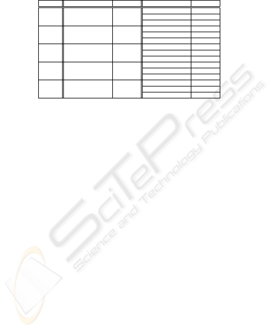
Table 1: Experimental results on the synthetic data set family.
Dataset Outlying subspace Outlier score Algorithm output Outlier score
0000100001 1.121307
Synth10D 0000100001 1.121307 0000100001 1.121307
0000100001 1.121307
101000010000 1.428615
Synth12D 101000010000 1.428615 101000010000 1.428615
101000010000 1.428615
000010011000000 1.522407
Synth15D 000010011000000 1.522407 000010011000000 1.522407
000010011000000 1.522407
000100000010001100 1.667848
Synth18D 000100000010001100 1.667848 000100000010001000 1.424176
000100000010001000 1.424176
00011000000001000010 1.701322
Synth20D 00011000000001000010 1.701322 00011000100001000011 0.995888
00011000000001000010 1.701322
this subspace, nine objects of the set DS
O
wdbc
belong
to the top twenty distance-based outliers of DS (that
is the 90%).
Thus, by exploiting our method we singled out a
subspace in which the anomalies detected by using
the distance-based definition are of better quality with
respect to those detected in the full feature space by
using the same definition.
5 CONCLUSIONS
We presented an example-based outlier detection
method exploiting both positive and negative exam-
ples in order to search for anomalies in an input data
set. The task here introduced is novel, in that previous
methods are able to exploit only positive examples,
and, moreover, are based on different outlier defini-
tions. We presented a subspace discovery algorithm
designed to search for the optimal subspace, and ex-
periments showed that the method is able to detect a
suboptimal solution, and that the method is promising
from the point of view of the knowledge mined.
As a future work, it is of interest to investigate
the inclusion in our framework of other outlier defini-
tions, and the design of policies for selecting outliers
in the outlying subspace guided by the examples. Fi-
nally, we plan to execute a more extensive experimen-
tal campaign concerning both from the computational
and the semantic point of view.
REFERENCES
Aggarwal, C. C. and Yu, P. (2001). Outlier detection for
high dimensional data. In Proc. Int. Conference on
Managment of Data.
Angiulli, F. and Pizzuti, C. (2002). Fast outlier detection in
large high-dimensional data sets. In Proc. Int. Conf. on
Principles of Data Mining and Knowledge Discovery,
pages 15–26.
Holland, J. (1992). Adaptation in Natural and Artificial Sys-
tems. The MIT Press, Cambridge, MA.
Holland, J., Holyoak, K., Nisbett, R., and Thagard, P.
(1986). Computational Models of Cognition and Per-
ception, chapter Induction: Processes of Inference,
Learning, and Discovery. The MIT Press, Cambridge,
MA.
Papadimitriou, S., Kitagawa, H., Gibbons, P. B., and Falout-
sos, C. (2003). Loci: Fast outlier detection using the
local correlation integral. In ICDE, pages 315–326.
Wei, L., Qian, W., Zhou, A., Jin, W., and Yu, J. (2003). Hot:
Hypergraph-based outlier test for categorical data. In
Proc. of the Pacific-Asia Conf. on Knowledge Discov-
ery and Data Mining, pages 399–410.
Zhang, J. and Wang, H. (2006). Detecting outlying sub-
spaces for high-dimensional data: the new task, algo-
rithms, and performance. Knowledge and Information
Systems, to appear.
Zhu, C., Kitagawa, H., and Faloutsos, C. (2005). Example-
based robust outlier detection in high dimensional
datasets. In Proc. Fifth IEEE International Confer-
ence on Data Mining, pages 829–832.
ICAART 2010 - 2nd International Conference on Agents and Artificial Intelligence
10