
SIMPLE GENETIC ALGORITHM WITH GENERALISED
α
⋆
-SELECTION
Dynamical System Model, Fixed Points, and Schemata
Andr´e Neubauer
Information Processing Systems Lab, M¨unster University of Applied Sciences
Stegerwaldstraße 39, D-48565 Steinfurt, Germany
Keywords:
Genetic algorithm, Dynamical system model, Random heuristic search, α-selection, Generalised α
⋆
-selection.
Abstract:
The dynamical system model proposed by VOSE provides a theory of genetic algorithms as specific random
heuristic search (RHS) algorithms by describing the stochastic trajectory of a population with the help of
a deterministic heuristic function and its fixed points. In order to simplify the mathematical analysis and to
enable the explicit calculation of the fixed points the simple genetic algorithm (SGA) with α-selection has been
introduced where the best or α-individual is mated with individuals randomly chosen from the population with
uniform probability. This selection scheme also allows to derive a simple coarse-grained system model based
on the equivalence relation imposed by schemata.
In this paper, the α-selection scheme is generalised to α
⋆
-selection by allowing the β best individuals of the
current population instead of the single best α-individual to mate with other individuals randomly chosen
from the population. It is shown that most of the results obtained for α-selection can be transferred to the SGA
with generalised α
⋆
-selection, e.g. the explicit calculation of the fixed points of the heuristic function or the
derivation of a coarse-grained system model based on schemata.
1 INTRODUCTION
As specific instances of random heuristic search
(RHS), genetic algorithms mimic biological evolu-
tion and molecular genetics in simplified form. Ge-
netic algorithms process populations of individuals
which evolve according to selection and genetic op-
erators like crossover and mutation. The algorithm’s
stochastic dynamics can be described with the help
of a dynamical system model introduced by VOSE
et al. (Reeves and Rowe, 2003; Vose, 1999a; Vose,
1999b). The population trajectory is attracted by the
fixed points of an underlying deterministic heuristic
function which also yields the expected next popula-
tion. However, even for moderate problem sizes the
calculation of the fixed points is difficult.
The simple genetic algorithm (SGA) with α-
selection allows to explicitly derive the fixed points
of the heuristic function as well as to formulate a
simple coarse-grained system model based on the
equivalence relation imposed by schemata (Neubauer,
2008a; Neubauer, 2008b). In this selection scheme,
the best or α-individual is mated with individuals ran-
domly chosen from the current population with uni-
form probability. This paper extends the α-selection
scheme to generalised α
⋆
-selection by allowing the
β best individuals of the current population instead
of the single best α-individual to mate with other in-
dividuals randomly chosen from the current popula-
tion. It is shown that most results obtained for the
SGA with α-selection can be transferred to the SGA
with generalised α
⋆
-selection by redefining the sys-
tem matrix of the dynamical system model, e.g. the
explicit calculation of the fixed points of the respec-
tive heuristic function or the derivation of a simple
coarse-grained system model based on schemata.
The paper is organised as follows. In section 2, the
SGA with α-selection is defined, the dynamical sys-
tem model, the corresponding heuristic function and
its fixed points are formulated, and a simple coarse-
grained system model based on the equivalence rela-
tion imposed by schemata is described. In section 3,
these results are extended to the SGA with generalised
α
⋆
-selection. A brief conclusion is given in section 4.
204
Neubauer A. (2009).
SIMPLE GENETIC ALGORITHM WITH GENERALISED a*-SELECTION - Dynamical System Model, Fixed Points, and Schemata.
In Proceedings of the International Joint Conference on Computational Intelligence, pages 203-208
DOI: 10.5220/0002312602030208
Copyright
c
SciTePress

2 SGA WITH α-SELECTION
The SGA with α-selection, crossover and mutation
defined by masks is described in this section follow-
ing (Neubauer, 2008a; Neubauer, 2008b) and the no-
tation and definition of the SGA in (Vose, 1999a).
In the present context, the genetic algorithm is used
for the maximisation of a fitness function f : Ω → R
which is defined over the search space Ω = Z
ℓ
2
=
{0,1}
ℓ
. Each binary ℓ-tuple (a
0
,a
1
,... , a
ℓ−1
) will
be identified with the integer a = a
0
· 2
ℓ−1
+ a
1
·
2
ℓ−2
+ ... + a
ℓ−1
· 2
0
leading to the search space
Ω = {0,1,..., n − 1} with cardinality |Ω| = n = 2
ℓ
.
With this binary number representation, the bitwise
modulo-2 addition a⊕b, modulo-2 multiplication a⊗
b and binary complement a are defined. The integer a
is also viewed as a column vector (a
0
,a
1
,... , a
ℓ−1
)
T
;
the integer n − 1 = 2
ℓ
− 1 corresponds to the all-one
ℓ-tuple 1. Finally, the indicator function [i = j] is de-
fined by [i = j] = 1 if i = j and 0 if i 6= j.
The SGA with α-selection formulated in
(Neubauer, 2008a; Neubauer, 2008b) works over
populations of r individual binary ℓ-tuples a ∈ Ω. In
each generation, offspring individuals are generated
by genetic operators like crossover χ
Ω
and mutation
µ
Ω
which are applied to selected parental individuals.
In the α-selection scheme, the best individual or
α-individual b in the current population is mated
with individuals randomly chosen from the current
population with uniform probability r
−1
(see Fig. 1).
initialise population;
while end of iteration 6= true do
select α-individual b as first parent;
for the creation of r offspring do
select second parent c randomly;
create offspring a = µ
Ω
(χ
Ω
(b,c));
end
end
Figure 1: SGA with α-selection.
The crossover operator χ
Ω
: Ω× Ω → Ω randomly
generates an offspring ℓ-tuple a = (a
0
,a
1
,... , a
ℓ−1
)
according to a = χ
Ω
(b,c) with crossover probabil-
ity χ from two ℓ-tuples b = (b
0
,b
1
,... , b
ℓ−1
) and
c = (c
0
,c
1
,... , c
ℓ−1
). With the crossover mask m ∈ Ω
the ℓ-tuples a = b⊗ m⊕ m⊗ c or a = b ⊗ m⊕ m⊗ c
are generated one of which is chosen as offspring a
with equal probability 2
−1
. The crossover mask m is
randomly chosen from Ω according to the probability
distribution vector χ = (χ
0
,χ
1
,... , χ
n−1
)
T
.
The mutation operator µ
Ω
: Ω → Ω randomly flips
each bit of the ℓ-tuple a = (a
0
,a
1
,... , a
ℓ−1
) with mu-
tation probability µ. It can be equivalently formulated
with the help of the mutation mask m ∈ Ω according
to µ
Ω
(a) = a⊕ m. The mutation mask m is randomly
chosen from Ω according to the probability distribu-
tion vector µ = (µ
0
,µ
1
,... , µ
n−1
)
T
.
2.1 Dynamical System Model
The dynamical system model of the SGA with
α-selection can be compactly formulated with the
population vector p = (p
0
, p
1
,... , p
n−1
)
T
. Each
component p
i
gives the proportion of element
i ∈ Ω in the current population. The popula-
tion vector p is an element of the simplex Λ =
{p ∈ R
n
: p
i
≥ 0∧
∑
i∈Ω
p
i
= 1}.
The SGA with α-selection is an instance of RHS
τ : Λ → Λ. The RHS τ is equivalently represented by
a heuristic function G : Λ → Λ according to q = τ(p)
with the expected next generation population vec-
tor q (see Fig. 2). For a given population vector p
the heuristic function G yields the probability distri-
bution G (p)
i
= Pr{individual i is sampled from Ω}
which underlies the generation of the next population.
The stochastic trajectory p, τ(p), τ
2
(p), ... approx-
imately follows the trajectory p, G (p), G
2
(p), ...
of the deterministic dynamical system defined by G .
The RHS τ behaves like the dynamical system model
in the limit of infinite populations (Vose, 1999a).
p
q = G (p)
G
Figure 2: Dynamical system model of the SGA.
2.1.1 Heuristic
In the α-selection scheme, the α-individual b is se-
lected as the first parent whereas the second parent is
chosen uniformly at random from the current popu-
lation. The heuristic function G (p) is then given by
(Neubauer, 2008a; Neubauer, 2008b)
q = G (p) = A· p (1)
with the system matrix
A = σ
b
· M
∗
· σ
b
. (2)
Here, (σ
b
)
i, j
= [i ⊕ j = b] denotes the permutation
matrix. The n × n mixing matrix is defined by (Vose,
1999a)
M
i, j
=
∑
u,v∈Ω
µ
v
·
χ
u
+ χ
u
2
· [i ⊗ u⊕ u⊗ j = v] . (3)
The twist M
∗
of the symmetric mixing matrix M =
M
T
is given by (M
∗
)
i, j
= M
i⊕ j,i
. The components of
the n× n system matrix are given by
SIMPLE GENETIC ALGORITHM WITH GENERALISED a*-SELECTION - Dynamical System Model, Fixed Points,
and Schemata
205

A
i, j
= M
i⊕b,i⊕ j
. (4)
Compared to the SGA in (Vose, 1999a), the α-
selection scheme yields a simpler heuristic function
G which is completely described by the α-individual
b and the mixing matrix M. This dynamical system
model is illustrated in Fig. 3.
p
q
σ
b
M
∗
σ
b
Figure 3: Dynamical system model of the SGA with α-
selection.
2.1.2 Fixed Points
For a given α-individual b the heuristic function
G (p) = A · p of the SGA with α-selection is linear.
The fixed points ω = G (ω) = A·ω are obtained from
the eigenvectors of the system matrix A to eigenvalue
1. There exists a single eigenvalue λ
0
= 1 with corre-
sponding eigenvector ω whereas the remaining n − 1
eigenvalues fulfill 0 ≤ λ
i
≤ 1− 2µ. The eigenvector ω
yields the unique fixed point of the heuristic function
G for a given α-individual b.
The fixed point ω can be determined explicitly
with the help of the WALSH transform. For the ma-
trix A the WALSH transform is
b
A = W · A · W with
the symmetric and orthogonal n × n WALSH matrix
W
i, j
= n
−1/2
· (−1)
i
T
j
(Vose and Wright, 1998). The
WALSH transform of the vector ω is
b
ω = W · ω. A
and its WALSH transform
b
A have the same eigenval-
ues with eigenvectors which are also related by the
WALSH transform, especially yielding ω = A · ω ⇔
b
ω =
b
A·
b
ω. The WALSH transform of the system ma-
trix is given by
b
A
i, j
=
b
M
i⊕ j, j
· (− 1)
b
T
(i⊕ j)
. (5)
For 1-point crossover χ
Ω
and mutation µ
Ω
the
WALSH transform of the mixing matrix M is formu-
lated in (Vose, 1999a). Because the WALSH trans-
form of the mixing matrix fulfills
b
M
i, j
∝ [i ⊗ j = 0]
the WALSH transform
b
A is a lower triangular matrix
(Neubauer, 2008a; Neubauer,2008b). Due to the rela-
tion
b
ω =
b
A·
b
ω the WALSH transform of the fixed point
can be iteratively determined from
b
ω
i
=
1
1−
b
A
i,i
·
i−1
∑
j=0
b
A
i, j
·
b
ω
j
(6)
for 1 ≤ i ≤ n− 1 starting with
b
ω
0
= n
−1/2
which en-
sures
∑
i∈Ω
ω
i
= 1. The fixed point ω = W ·
b
ω is finally
obtained via the inverse WALSH transform.
2.2 Schemata
Following (Vose, 1999a) schemata can be considered
as specific equivalence relations in which two equiva-
lent individuals i ≡ j in the search space Ω belong to
the same equivalence class [i] = { j ∈ Ω : j ≡ i}. With
the help of the quotient map Ξ
[i], j
= [i ≡ j] this can be
expressed as i ≡ j if and only if Ξ
[i], j
= 1. Two popu-
lations are equivalent if the proportions of individuals
in each equivalence class [i] ∈ Ω/≡ with i ∈ Ω are the
same in both populations. With population vectors p
and p
′
this corresponds to the condition Ξp = Ξp
′
.
A schemata family is defined by the ℓ-tuple ξ ∈ Ω
via the quotient map Ξ
[i], j
= [ j⊗ ξ = i] with i ∈ Ω
ξ
=
{i ∈ Ω : i⊗ ξ = 0} and j ∈ Ω leading to the 2
1
T
ξ
× 2
ℓ
matrix Ξ. Two individuals i, j ∈ Ω are equivalent if
they agree on the defining positions of the schemata
family according to i ≡ j ⇔ i⊗ ξ = j ⊗ ξ. The cardi-
nality of Ω
ξ
is
Ω
ξ
= 2
1
T
ξ
with the number of defin-
ing positions 1
T
ξ.
2.2.1 Schema Heuristic
A dynamical system G is consistently modeled by
the simplified coarse-grained system
e
G implied by the
equivalence relation ≡ if the diagram in Fig. 4 com-
mutes, i.e. for two equivalent population vectors p and
p
′
the population vectors in the next generation G (p)
and G (p
′
) must also be equivalent.
p
G (p)
e
p
ΞG (p)
ΞΞ
G
e
G
Figure 4: Commutativity diagram with quotient map Ξ.
For the SGA with α-selection, crossover and mu-
tation the proportion of the expected next population
representing schema [i] = i⊕ Ω
ξ
with i ∈ Ω
ξ
is given
by (Neubauer, 2008a; Neubauer, 2008b)
ΞG(p) = A
ξ
· Ξp . (7)
The 2
1
T
ξ
× 2
1
T
ξ
schema system matrix
A
ξ
[i],[ j]
=
M
ξ
[i⊕b],[i⊕ j]
(8)
with i, j ∈ Ω
ξ
is defined with the help of the 2
1
T
ξ
×
IJCCI 2009 - International Joint Conference on Computational Intelligence
206
2
1
T
ξ
schema mixing matrix
M
ξ
[i],[ j]
=
∑
u,v∈Ω
ξ
(Ξµ)
[v]
·
(Ξχ)
[u]
+ (Ξχ)
[u]
2
·
[i⊗ u⊕ u⊗ j = v] . (9)
The schema system matrix A
ξ
can be obtained from
system matrix A and quotient map Ξ according to
A
ξ
=
2
1
T
ξ
n
· Ξ · A· Ξ
T
. (10)
The schema heuristic function
e
G is defined ac-
cording to
e
G (Ξp) = A
ξ
·Ξp. Since the schema system
matrix A
ξ
depends on the α-individual b the heuristic
function G is not compatible with the equivalence re-
lation imposed by schemata in the strict sense. If the
α-individual b is lost or a better individual is sam-
pled from the search space Ω in the next generation
the schema system matrix A
ξ
and the schema heuristic
function
e
G change. The α-individual b can be consid-
ered as an exogenous parameter to the coarse-grained
system model (see Fig. 5).
e
p
e
G (
e
p)
e
G
b
Figure 5: Coarse-grained system model of the SGA with
α-selection depending on the α-individual b.
2.2.2 Schema Fixed Points
As for the dynamical system model and the corre-
sponding heuristic function G , there exists a unique
fixed point of the schema heuristic function
e
G which
can be calculated from the WALSH transform
b
A
ξ
=
W
ξ
·A
ξ
·W
ξ
of the schema system matrix A
ξ
. Here, the
2
1
T
ξ
×2
1
T
ξ
WALSH matrix W
ξ
is defined over Ω
ξ
. The
WALSH transform
b
A
ξ
of the schema system matrix A
ξ
is given by
(
b
A
ξ
)
[i],[ j]
= (
b
M
ξ
)
[i⊕ j],[ j]
· (− 1)
b
T
(i⊕ j)
(11)
with i, j ∈ Ω
ξ
.
b
A
ξ
is obtained from
b
A by choosing
rows and columns with indices in Ω
ξ
, i.e.
(
b
A
ξ
)
[i],[ j]
=
b
A
i, j
. (12)
Similar to the system matrix A it can be shown that
the WALSH transform
b
A
ξ
of the schema system ma-
trix A
ξ
is a lower triangular matrix with an eigenvalue
λ
[0]
= (
b
A
ξ
)
[0],[0]
= 1 leading to the unique schema
fixed point
e
ω = A
ξ
·
e
ω which is related to the fixed
point ω according to
e
ω = Ξω. Taking into account
b
e
ω =
b
A
ξ
·
b
e
ω the WALSH transform of the schema fixed
point can be iteratively determined from
b
e
ω
[i]
=
1
1−
b
A
i,i
·
∑
j∈Ω
ξ
∩{0,1,...,i−1}
b
A
i, j
·
b
e
ω
[ j]
(13)
for i ∈ Ω
ξ
starting with
b
e
ω
[0]
= 2
−1
T
ξ/2
. The schema
fixed point
e
ω = W
ξ
·
b
e
ω is finally obtained via the in-
verse WALSH transform over Ω
ξ
.
3 SGA WITH GENERALISED
α
⋆
-SELECTION
The α-selection scheme can be generalised by allow-
ing the β best individuals of the current population
instead of the single best α-individual to mate with
other individuals randomly chosen from the current
population. Most of the theoretical results obtained
for α-selection with a single α-individual are trans-
ferrable to the SGA with generalised α
⋆
-selection.
The SGA with generalised α
⋆
-selection is illus-
trated in Fig. 6. For the generalised α
⋆
-selection
scheme the β best individuals b
0
, b
1
, .. ., b
β−1
in
the current population are mated with individuals ran-
domly chosen from the current population. For the
creation of each offspring individual one of the β best
individuals b
0
, b
1
, ..., b
β−1
is chosen with uniform
probability β
−1
as the first parent b whereas the sec-
ond parent c is chosen uniformly at random from the
current population with probability r
−1
.
initialise population;
while end of iteration 6= true do
select β best individuals b
0
, b
1
, ..., b
β−1
;
for the creation of r offspring do
select first parent b from β
best individuals randomly;
select second parent c from
population randomly;
create offspring a = µ
Ω
(χ
Ω
(b,c));
end
end
Figure 6: SGA with generalised α
⋆
-selection.
SIMPLE GENETIC ALGORITHM WITH GENERALISED a*-SELECTION - Dynamical System Model, Fixed Points,
and Schemata
207

3.1 Dynamical System Model
In this section, the dynamical system model, the cor-
responding heuristic function and its fixed points are
derived for the SGA with generalised α
⋆
-selection.
3.1.1 Heuristic
In the generalised α
⋆
-selection scheme, one of the β
best individuals is selected from the set {b
k
}
0≤k≤β−1
as the first parent with uniform probability β
−1
whereas the second parent is chosen uniformly at ran-
dom from the current population according to the
probability distribution Pr{individual j is selected} =
p
j
with j ∈ Ω. The heuristic function G is given by
G (p)
i
=
β−1
∑
k=0
1
β
n−1
∑
j=0
p
j
· Pr{µ
Ω
(χ
Ω
(b
k
, j)) = i} .
The mixing operation comprises crossover χ
Ω
and
mutation µ
Ω
. With the help of the probability distri-
butions for crossover and mutation this leads to
Pr{µ
Ω
(χ
Ω
(b
k
, j)) = i}
=
∑
u∈Ω
µ
u
· Pr{χ
Ω
(b
k
, j) = i⊕ u}
=
∑
u∈Ω
µ
u
∑
v∈Ω
χ
v
+ χ
v
2
· [b
k
⊗ v⊕ v⊗ j = i⊕ u]
= M
i⊕b
k
,i⊕ j
with n × n mixing matrix M according to (3). The
heuristic function is
G (p)
i
=
n−1
∑
j=0
p
j
·
1
β
β−1
∑
k=0
M
i⊕b
k
,i⊕ j
.
With the n× n system matrix
A
i, j
=
1
β
β−1
∑
k=0
M
i⊕b
k
,i⊕ j
(14)
this leads to the linear system of equations for the ex-
pected next population vector
q
i
= G (p)
i
=
n−1
∑
j=0
A
i, j
· p
j
(15)
or equivalently
q = G (p) = A· p (16)
which corresponds to the heuristic function in (1) for
the SGA with α-selection. By making use of the per-
mutation matrix σ
b
and the twist M
∗
of the mixing
matrix the system matrix A can be expressed as
A =
1
β
β−1
∑
k=0
σ
b
k
· M
∗
· σ
b
k
. (17)
The corresponding dynamical system model is illus-
trated in Fig. 7.
p
q
σ
b
0
M
∗
σ
b
0
σ
b
1
M
∗
σ
b
1
σ
b
β−1
M
∗
σ
b
β−1
.
.
.
.
.
.
.
.
.
β
−1
+ ×
Figure 7: Dynamical system model of the SGA with gener-
alised α
⋆
-selection.
3.1.2 Fixed Points
Similar to the SGA with α-selection the fixed points
ω of the heuristic function G are obtained from the
eigenvectors of the system matrix A to eigenvalue 1
due to the linear relation G (p) = A· p for a given set
{b
k
}
0≤k≤β−1
of β best individuals. Since the system
matrix A and its WALSH transform
b
A have the same
eigenvalues with eigenvectors, which are also related
by the WALSH transform, the WALSH transform of
the system matrix
b
A
i, j
=
b
M
i⊕ j, j
·
1
β
β−1
∑
k=0
(−1)
b
T
k
(i⊕ j)
(18)
is derived. The system matrix A as well as its WALSH
transform
b
A depend on the β best individuals.
The WALSH transform
b
A is a lower triangular ma-
trix with eigenvalues λ
i
given by the diagonal ele-
ments λ
i
=
b
A
i,i
=
b
M
0,i
leading to
λ
i
=
(1− 2µ)
1
T
i
2
·
∑
k∈Ω
i
(χ
k
+ χ
k⊕i
) . (19)
Because of λ
0
= 1 and 0 ≤ λ
i
≤ 1 − 2µ for 1 ≤ i ≤
n− 1 there exists a single eigenvector ω to eigenvalue
1 which is a fixed point of the heuristic function ω =
G (ω) = A· ω. Taking into account
b
ω =
b
A ·
b
ω with
lower triangular matrix
b
A the WALSH transform
b
ω of
the fixed point can be recursively calculated according
to (6). The fixed point is then obtained via the inverse
WALSH transform ω = W ·
b
ω.
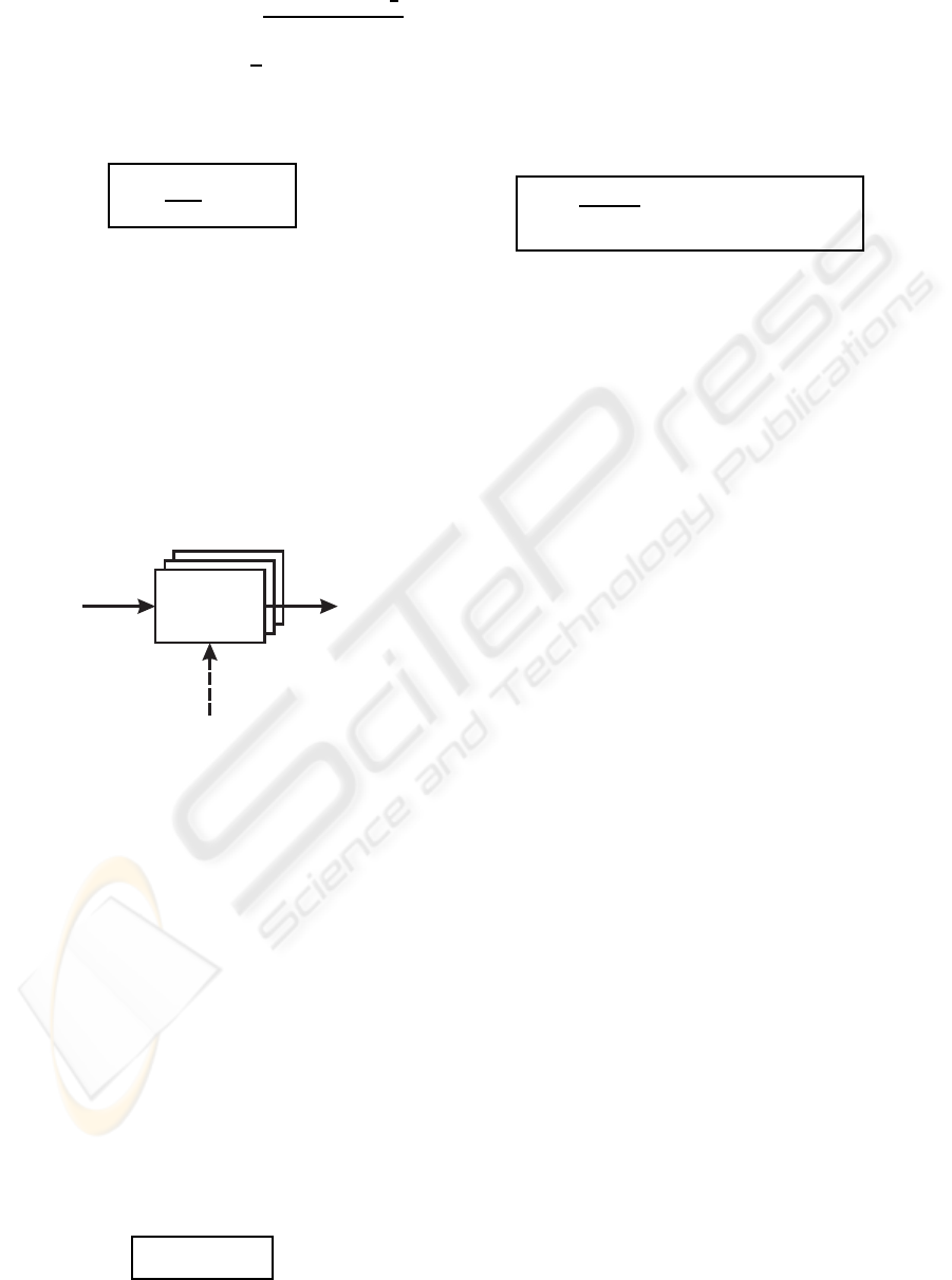
3.2 Schemata
In correspondence to the SGA with α-selection, the
schema heuristic function will be formulated for the
SGA with generalised α
⋆
-selection in this section.
3.2.1 Schema Heuristic
The proportion of the expected next population repre-
senting schema [i] = i⊕ Ω
ξ
with i ∈ Ω
ξ
is given by
ΞG(p) = A
ξ
· Ξp . (20)
IJCCI 2009 - International Joint Conference on Computational Intelligence
208

The 2
1
T
ξ
× 2
1
T
ξ
schema system matrix is defined by
A
ξ
[i],[ j]
=
1
β
β−1
∑
k=0
M
ξ
[i⊕b
k
],[i⊕ j]
(21)
with i, j ∈ Ω
ξ
and the 2
1
T
ξ
× 2
1
T
ξ
schema mixing ma-
trix M
ξ
defined in (9). As in (10), the schema system
matrix A
ξ
can be obtained from system matrix A and
quotient map Ξ.
The schema system matrix A
ξ
and the schema
heuristic function
e
G defined by
e
G (Ξp) = A
ξ
· Ξp de-
pend on the set {b
k
}
0≤k≤β−1
of β best individuals.
This set (or the set {[b
k
]}
0≤k≤β−1
of their correspond-
ing equivalence classes) thus acts like an exogenous
parameter set to the coarse-grained system model, as
illustrated in Fig. 8.
e
p
e
G (
e
p)
e
G
{b
k
}
0≤k≤β−1
Figure 8: Coarse-grained system model of the SGA with
generalised α
⋆
-selection.
3.2.2 Schema Fixed Points
For a given set {b
k
}
0≤k≤β−1
of β best individuals
there exists a unique fixed point of the schema heuris-
tic function
e
G which again can be calculated from the
WALSH transform
b
A
ξ
of the schema system matrix A
ξ
which is given by
(
b
A
ξ
)
[i],[ j]
= (
b
M
ξ
)
[i⊕ j],[ j]
·
1
β
β−1
∑
k=0
(−1)
b
T
k
(i⊕ j)
(22)
with i, j ∈ Ω
ξ
. As for the SGA with α-selection,
b
A
ξ
is obtained from
b
A by choosing rows and columns
with indices in Ω
ξ
according to (12). By exploiting
the lower triangularity of the WALSH transform
b
A
ξ
of
the schema system matrix A
ξ
and the existence of an
eigenvalue λ
[0]
= (
b
A
ξ
)
[0],[0]
= 1 the schema fixed point
e
ω = A
ξ
·
e
ω can be determined as in (13).
e
ω can also be
obtained from the fixed point ω according to
e
ω = Ξω.
4 CONCLUSIONS
The dynamical system model describes the stochastic
dynamics of genetic algorithms with the help of the
deterministic heuristic function G and its fixed points.
Since for practical problem sizes the calculation of
the fixed points is difficult the SGA with α-selection
has been introduced in (Neubauer, 2008a; Neubauer,
2008b). For a given α-individual b the heuristic func-
tion G of the SGA with α-selection is defined by a
linear system of equations with system matrix A. The
unique fixed point ω can be calculated analytically
from the WALSH transformed system matrix
b
A.
As is shown in this paper, the theoretical re-
sults obtained for the SGA with α-selection can be
transferred to the SGA with generalised α
⋆
-selection.
In this selection scheme, the β best individuals of
the current population instead of the single best α-
individual mate with other individuals randomly cho-
sen from the current population. Generalised α
⋆
-
selection with β > 1 represents a weaker selection
scheme than α-selection in the sense that not only the
best individual b is used as the first parent but the β
best individuals b
0
, b
1
, ..., b
β−1
are allowed to repro-
duce as the first parent. For a given set {b
k
}
0≤k≤β−1
of β best individuals the heuristic function G of the
SGA with generalised α
⋆
-selection is also formulated
by a linear system of equations with a suitably re-
defined system matrix A. As for the SGA with α-
selection, the SGA with generalised α
⋆
-selection al-
lows to explicitly determine a simple coarse-grained
system model for a schemata family defined by the
ℓ-tuple ξ. The corresponding RHS is defined by the
schema system matrix A
ξ
with similar properties as
the system matrix A.
REFERENCES
Neubauer, A. (2008a). Intrinsic system model of the genetic
algorithm with α-selection. In Parallel Problem Solv-
ing from Nature PPSN X, Lecture Notes in Computer
Science, pages 940–949. Springer.
Neubauer, A. (2008b). Theory of the simple genetic algo-
rithm with α-selection. In Proceedings of the 10th
Annual Genetic and Evolutionary Computation Con-
ference – GECCO 2008, pages 1009–1016.
Reeves, C. R. and Rowe, J. E. (2003). Genetic Algorithms
– Principles and Perspectives, A Guide to GA Theory.
Kluwer Academic Publishers, Boston.
Vose, M. D. (1999a). Random heuristic search. Theoretical
Computer Science, 229(1-2):103–142.
Vose, M. D. (1999b). The Simple Genetic Algorithm – Foun-
dations and Theory. MIT Press, Cambridge.
Vose, M. D. and Wright, A. H. (1998). The simple ge-
netic algorithm and the walsh transform – part i, the-
ory – part ii, the inverse. Evolutionary Computation,
6(3):253–273, 275–289.
SIMPLE GENETIC ALGORITHM WITH GENERALISED a*-SELECTION - Dynamical System Model, Fixed Points,
and Schemata
209
