ARTIFICIAL DATA GENERATION FOR ONE-CLASS

CLASSIFICATION

A Case Study of Dimensionality Reduction for Text and Biological Data

Santiago D. Villalba and P

adraig Cunningham

School of Computer Science and Informatics, University College Dublin, Ireland

Keywords:

Dimensionality reduction, One-class classiﬁcation, Novelty detection, Locality preserving projections, Text

classiﬁcation, Functional genomics.

Abstract:

Artiﬁcial negatives have been employed in a variety of contexts in machine learning to overcome data avail-

ability problems. In this paper we explore the use of artiﬁcial negatives for dimension reduction in one-class

classiﬁcation, that is classiﬁcation problems where only positive examples are available for training. We

present four different strategies for generating artiﬁcial negatives and show that two of these strategies are

very effective for discovering discriminating projections on the data, i.e., low dimension projections for dis-

criminating between positive and real negative examples. The paper concludes with an assessment of the

selection bias of this approach to dimension reduction for one-class classiﬁcation.

1 INTRODUCTION

Sometimes in practical classiﬁcation problems we are

given a sample in which only one of the classes, typ-

ically called the “positive” or “target” class, is well

represented, while the examples for the other classes

are not statistically representative or simply do not ex-

ist. That can be the case when the negatives space is

too broad (e.g., the writings of Cervantes against any

other possible writing), when it is expensive to label

the negatives (e.g., multimedia annotation) or when

negative examples have not yet arisen (e.g., industrial

process monitoring). In these cases building a dis-

criminative model using the ill-deﬁned negatives sam-

ple will lead to very poor generalization performance

and therefore conventional supervised techniques are

not appropriate (when usable).

One-class classiﬁcation (OCC) techniques (Tax,

2001), designed to construct discriminative models

when the training sample is representative of only one

of the classes, emerge as a solution to this kind of

problem. The difference is operational, while the task

is still to accept or reject unseen examples, this can

be done only based on their similarity to the known

positives. Consequently OCC approaches can oper-

ate with no or very few negative training examples,

handling the “no-counter-example” and “imbalanced-

data” problems by considering only positive data.

Many of the domains where one-class classiﬁca-

tion is appealing are characterized by high dimen-

sional datasets. This high dimensionality poses sev-

eral challenges to the learning system and so dimen-

sionality reduction becomes desirable. In this paper

we propose a simple technique that aims to introduce

a discriminative bias in dimensionality reduction for

one-class classiﬁcation. The algorithm is as follows:

1- enrich the training set by creating a second sample

that will act as a contrast for the actual positives 2- ap-

ply dimensionality reduction in the enriched dataset

and 3- use the low-dimensional representation found

to train a one-class classiﬁer. This idea follows a re-

cent trend in the relevant literature where OCC is cast

as a conventional supervised problem by sampling

artiﬁcial negatives from a reference distribution (see

section 3). In this way we try to bridge the gap be-

tween supervised classiﬁcation and one-class classiﬁ-

cation

However, the gap is wide. Formally when tack-

ling the classiﬁcation task in a supervised way we

are given a training set Z = {z

(1)

, . . . , z

(n)

} where

(i)

= (x

(i)

, y

(i)

) is an input-output pair, x

(i)

∈ X is

an input example and y

(i)

∈ Y is its associated out-

put from a set of classes. Usually X ⊆ R

so x

(i)

, x

, . . . , x

) is an m-dimensional real vector. Us-

ing Z we infer a classiﬁcation rule h ∈ H : X → Y

which maps inputs x to predicted outputs h(x) = ˆy ∈

Y . Given the usual 01 loss L

(h, x) = I( f (x) 6= y)

we are endeavor to ﬁnd

h that minimizes the risk

202

D. Villalba S. and Cunningham P. (2009).

ARTIFICIAL DATA GENERATION FOR ONE-CLASS CLASSIFICATION - A Case Study of Dimensionality Reduction for Text and Biological Data.

In Proceedings of the International Conference on Knowledge Discovery and Information Retrieval, pages 202-210

DOI: 10.5220/0002310202020210

 SciTePress

functional R(h) =

(h, x)p(x)dx. The primary as-

sumption in this learning setting is that Z is represen-

tative of the concept to be learnt, in this case the clas-

siﬁcation rule, which means that both the distribution

of the inputs p(x) and the conditional distribution of

the classes given the inputs p(y|x) can be estimated

from Z.

Conceptually one-class classiﬁcation is very at-

tractive. In practice it is very hard. Due to the absence

of a well-sampled second class, the learning system

cannot get comprehensive feedback and therefore un-

certainty governs the whole process. The fundamen-

tal machine learning assumption that the training set

is representative of the concept to be learnt does not

hold and by deﬁnition neither p(x) nor p(y|x) can be

estimated. From an OCC perspective we call the in-

complete information on p(x) the lack of Knowledge

of the Inputs Distribution (KID). The incomplete in-

formation on p(y|x) means we lack an Estimatable

Loss Function (ELF) that might be used in parameter

setting or model selection.

The rest of the paper is organized as follows. In

section 2 we introduce the problem of dimensional-

ity reduction in OCC and describe Locality Preserv-

ing Projections, the dimension reduction technique

we will use in combination with our artiﬁcial sam-

ples. In section 3 we present a brief review of the rel-

evant literature for artiﬁcial negative generation and

describe four simple strategies for generating artiﬁ-

cial negatives. In section 4 we show the promising

results of our approach in a comprehensive set of text

classiﬁcation problems and a biological dataset. We

bring the paper to a conclusion in section 5.

2 DIMENSIONALITY

REDUCTION

2.1 Dimensionality Reduction for

One-Class Classiﬁcation

The curse of dimensionality poses several challenges

for data analysis tools (Franc¸ois, 2008). In practice,

one-class problems are typically of high dimension

so dimensionality reduction (DR) is an important pre-

processing step. In fact, the evaluation on text classi-

ﬁcation presented by Manevitz and Yousef (Manevitz

and Yousef, 2001) shows that one-class Support Vec-

tor Machine (SVM) performance is quite sensitive to

the number of features used. This contrasts with two-

class SVMs which are generally considered to be ro-

bust to high data dimensionality. Although the liter-

ature on the topic is quite sparse, it is necessary to

study methods for combating high dimensionally in

the one-class setting.

Using dimensionality reduction prior to one-class

classiﬁcation should follow this rationale: ﬁnd a dis-

criminative representation (by feature selection or

transformation) that will improve the classiﬁcation

performance of the model describing the positive

class. Due to the ELF problem, conventional super-

vised and semi-supervised DR techniques cannot be

used for one-class classiﬁcation. This is unfortunate

because, clearly, supervision is more effective at dis-

covering discriminative representations. On the other

hand, unsupervised alternatives, relying on assump-

tions like locality or variance preservation, can be ir-

relevant or even harmful for classiﬁcation, especially

in the absence of actual negatives.

Unsupervised techniques can prove very useful

when their bias are correct for the problem at hand

and are well synchronized with the classiﬁer being

used (Villalba and Cunningham, 2007). Conventional

techniques for unsupervised dimensionality reduction

can do so as a byproduct of the underlying assump-

tions, but the KID problem has an important impact

in their application. For example, consider the case

of principal components analysis (PCA), perhaps the

most popular feature transformation technique. PCA

ﬁnds decorrelated dimensions in which the data vari-

ance is large, that is, where the data has a large spread.

Theoretically spreading the data has nothing to do

with ﬁnding discriminative directions, yet there are

numerous scenarios where PCA enhances classiﬁca-

tion accuracy. However, based on geometrical intu-

itions and an assumption of solvability for the clas-

siﬁcation problem, we can distinguish two different

scenarios when predicting the effectiveness of PCA

for classiﬁcation – if it has access to positives only or

if it can see both positives and negatives.

This conjecture of solvability is based on this ob-

servation: in the real world, we will usually face types

of classiﬁcation problems where there will be class

separability in at least some subspace. Often sepa-

rability comes together with high variability between

the classes and so, with a large spread in the whole

data. If projecting into those discriminative subspaces

will spread the data as a side effect, in practice we

can take the reverse path and ﬁnd high variability sub-

spaces with the hope that they will lead to class sepa-

rability. See ﬁgure 1 for a toy example.

On the other hand, in the pure one-class setting,

with no negatives at all at training time, spreading the

data can be regarded as a bad idea. Because of our

total ignorance of the negatives, the approach should

be to maximize the chance that, whatever is their dis-

tribution, we will accept as few of them as possible.

ARTIFICIAL DATA GENERATION FOR ONE-CLASS CLASSIFICATION - A Case Study of Dimensionality Reduction

for Text and Biological Data

203

-5 -4 -3 -2 -1 0 1 2 3 4 5

-10

-8

-6

-4

-2

86%

-5 -4 -3 -2 -1 0 1 2 3 4 5

-10

-8

-6

-4

-2

76%

-5 -4 -3 -2 -1 0 1 2 3 4 5

-10

-8

-6

-4

-2

52%

-5 -4 -3 -2 -1 0 1 2 3 4 5

-10

-8

-6

-4

-2

63%

Figure 1: PCA over an artiﬁcial 2-dimensional example.

We generate three mirroring data clouds by sampling from

Gaussian distributions with diagonal covariance, the vari-

ance in x

(“horizontal dimension”) is three times that in x

(“vertical dimension”), and the means differ only in x

. We

label the central cloud as the positives examples and the up-

per and lower clouds as the negatives, where the total num-

ber of positives and negatives is the same. When computing

PCA only with the positive data, the ﬁrst principal compo-

nent is x

, accounting for a 75% of the variance. This is

clearly a bad option. On the right side of each plot we indi-

cate the direction of the ﬁrst principal component found by

using both positives and negatives, labelled with the amount

of variance it accounts for. We move the negative clouds

so that they get closer and, eventually, overlap the positive

cloud. In this case PCA ﬁnds ”the right direction” until it is

no longer possible to do so because both classes overlap.

This is achieved by projections that make the positive

data occupy as little space as possible (collapsing),

which in PCA corresponds to those explaining less

variance (Tax and Muller, 2003).

In previous experiments with a wide range of high

dimensional datasets, PCA was found, indeed, not

as useful in a setting without actual negatives (Vil-

lalba and Cunningham, 2007). It can still help when

the aim is to reduce the dimensionality while keep-

ing as much information as possible, but the discrim-

inative aspect that emanates from class separability

completely disappears when training with just one

class. Related to the KID problem, the usefulness of

unlabeled data in classiﬁcation is one of the central

questions of the semi-supervised approach to learn-

ing (Chapelle et al., 2006, sect. 1.2); while in semi-

supervised classiﬁcation the effect of unlabeled data

can be negligible from a theoretical point of view, un-

labeled data plays a principal role in semi-supervised

one-class classiﬁcation (Scott and Blanchard, 2009).

2.2 Locality Preserving Projections

In this paper we focus on the interactions between

one-class classiﬁcation and Locality Preserving Pro-

jections (LPP) (He and Niyogi, 2003). LPP belongs

to the family of spectral methods, where the low di-

mensional representations are derived from the eigen-

vectors of specially constructed matrices. The idea

behind LPP is that of ﬁnding subspaces which pre-

serve the local structure in the data. LPP has its roots

in spectral graph theory (Chung, 1997), and the algo-

rithmic details along with the speciﬁc setup used in

our experiments are as follows:

1. Construct the Adjacency Graph: let X be the

training set and G denote a graph with n nodes.

We put an edge between nodes i and j if x

(i)

and

( j)

are “close”. When mixing with artiﬁcial gen-

eration techniques (sec. 3) we use a supervised

k-nearest neighbors approach, where nodes i and

j are connected if i is among the k-nearest neigh-

bors of j or vice-versa and y

(i)

= y

( j)

, that is, we

only allow links between examples of the same

class. We also use self-connected graphs.

2. Choose the Weights for the Graph Edges. W

is the adjacency matrix of G, a symmetric n × n

matrix with W

i j

having the weights of the edge

joining vertices i and j, and 0 if there is no such

edge. In this paper we use the simple approach of

putting W

i j

= 1 when nodes i and j are connected.

3. Eigenmaps. Compute the eigenvectors and

eigenvalues for the generalized eigenvector prob-

lem:

XLX

e = λXDX

e (1)

where D is a the degree matrix and L is the Lapla-

cian matrix (Chung, 1997). The embedding is de-

ﬁned by the bottom eigenvectors in the solution of

Equation 1.

It can be shown that by solving 1 we ﬁnd the direc-

tion e that minimizes

∑

i, j

(i)

− e

(j)

)

i j

. This

objective function incurs a high penalty if neighbor

points x

(i)

and x

( j)

are mapped far apart. Therefore

the bias of LPP is that of collapsing neighbor points.

This seems appropriate for one-class classiﬁcation,

where collapsing the target class so that it occupies

as little space as possible should account for many

“attacking” distributions. LPP can prove effective for

one-class classiﬁcation in domains with high redun-

dancy and low irrelevancy between dimensions, for

example chemical spectra or data coming from multi-

ple sensors. However, when using LPP with one-class

classiﬁcation we still miss the discriminative aspect,

so we will be collapsing neighborhoods inside the tar-

get class without necessarily creating a discriminating

representation.

KDIR 2009 - International Conference on Knowledge Discovery and Information Retrieval

204

3 ARTIFICIAL NEGATIVES

GENERATION

A possible solution to incorporate a discriminative

bias into OCC is to constrain the nature of the neg-

atives by studying what are the relevant negative dis-

tributions that can appear in practice. In this way, we

could generate artiﬁcial negatives (ANG) that could

be used to help train the system. Our data would then

come from a mixture distribution Q :

X ∼ Q = (1 − π)P + πA (2)

where P is the distribution for the positives, A is the

assumed distribution for the negatives and π ∈ [0, 1]

controls their proportion. Paradoxically, with this ap-

proach the distribution we know is that of the nega-

tives while P is to be estimated from data.

This notion of arbitrarily generating negative data

to enable the application of supervised techniques in

unsupervised problems seems very na

ıve, but it is ad-

vocated by well respected statisticians (Hastie et al.,

2001, pg. 449). Recent theoretical studies in one-

class classiﬁcation also provide justiﬁcation for this

approach. El-Yaniv and Nisenson study the decision

aspect of one-class classiﬁcation, when to accept a

new example, in an hypothetical setting where P is

fully known (El-Yaniv and Nisenson, 2006). Using a

game-theoretic, “foiling the adversary” analysis, they

conclude that the optimal strategy to deal with an un-

known “attacking distribution” is to use randomiza-

tion at the decision level (i.e., incorporate a random

element in the classiﬁer outputs). They also justify the

common heuristic of using the uniform for A, when

deﬁning negatives as examples in low density areas of

positives, as a worst-case attacking distribution in this

scenario.

Estimating density level sets has been cast as su-

pervised problems with contrasting examples sam-

pled from a reference distribution (Scott and Nowak,

2006; Steinwart et al., 2005). Again, these are applied

to one-class classiﬁcation by deﬁning negatives as ex-

amples in low density areas. Related heuristics have

been used in one-class classiﬁcation for tasks such as

model selection by volume estimation (Tax and Duin,

2002). These use the volume as a proxy to estimate

the error. Other fully supervised approaches for one-

class classiﬁcation by the generation of artiﬁcial neg-

ative samples and the use of supervised classiﬁers can

also be found in the literature (Fan et al., 2004; Abe

et al., 2006).

3.1 Non-parametric Artiﬁcial Negatives

Generation

Actual negatives could live anywhere in the input

space, thus the space of actual classiﬁcation problems

for a given set of positive data samples is very large.

In high dimensional spaces, we can generate nega-

tives anywhere and the generation method chosen will

bias the resulting classiﬁer. So the question is, what

are appropriate principles to drive the generation pro-

cess?

Ultimately we want to train a classiﬁer that will

be prepared for mischievous and adversarial attacking

distributions of negatives. A principled way to do that

is to try to generate negatives that resemble the pos-

itives - mimicking some aspects found in P - as that

will create hard but solvable problems. By solvable

we mean that there should be a way of discriminat-

ing P from A, while by hard we mean, for example,

looking for boundary cases or for negative samples

in which the correlations between the features present

in the positives are kept. In layman terms, our moti-

vation is to generate artiﬁcial negatives that look like

the positives without being positives so that the dis-

criminating dimensions that are chosen stress the real

essence of the positives.

In fact, for the ANG based technique proposed

in (Hempstalk et al., 2008) it is shown that an ideal

solution is to generate negatives by sampling from

the very same distribution of the positives. Paramet-

ric models ﬁtted to the positives (e.g., a Multivariate

Gaussian) could be a useful ANG. However, in high-

dimensional spaces ﬁtting a parametric model seems

futile. Therefore we turn our attention towards non-

parametric and geometrically motivated ANG tech-

niques. The following are four simple methods for

generating artiﬁcial negatives:

Uniform. Negatives coming from the uniform distri-

bution are commonly used in the literature. As indi-

cated previously, the rationale for sampling the nega-

tives from the uniform is that of low-density rejection.

This method can perform poorly when the distribu-

tion of the actual negatives is far from uniform while

still having a big overlap with P (Scott and Blanchard,

2009), and it has important computational problems

when trying to cover high dimensional spaces.

Marginal. Generating negatives by random sam-

pling from the empirical marginal distribution of the

positives, that is, to randomly permute the values

within each feature, breaks the correlation between

the features while maintaining the artiﬁcial negatives

in dense areas of positives (Francois et al., 2007).

Breiman and Cutler, in their random forest implemen-

ARTIFICIAL DATA GENERATION FOR ONE-CLASS CLASSIFICATION - A Case Study of Dimensionality Reduction

for Text and Biological Data

205

tation (Breiman, 2001), apply this method to allow

the construction of forests which, as a byproduct, pro-

duce an emergent measure of proximities between ex-

amples and a ranking of features (Shi and Horvath,

2006).

Left-right. This method simple translates each ex-

ample in one of two directions, “left” or “right”. The

translation in each dimension depends on the ob-

served range of that dimension and is scaled by a

parameter ρ ∈ R, chosen a priori. Formally a

(i)

+ ρ

(i)

r, where r = (r

, r

, . . . , r

) is the vector of

features ranges (r

= |max(x

) − min(x

)|)and ρ

(i)

selected at random from −ρ (“to the left”) and ρ (“to

the right ”). See ﬁgure 2.

ρ = 1

ρ = 8

Figure 2: From the many directions possible, the LeftRight

generator displaces each positive point to the left (translate

each coordinate by a negative amount) or to the right (trans-

late each coordinate by a positive amount). By choosing to

translate in these two unique directions, we are generating

two clouds of points that are arbitrarily far from the original

sample of positives. Translation is an afﬁne transformation

and so all the distances ratios get preserved in each of the

two clouds, so each cloud accounts for a different stochas-

tic view of the neighborhoods present in the positives. This

gives different related goals for LPP and also forces it to

“collapse” the positives, as the graph W is made up of at

least three connected components that arise from analogous

clouds of points in the original Euclidean space. Our arbi-

trary choice to scale up the translation by the range in each

dimension makes the distances between clouds larger in di-

mensions with high variance, in this case z.

Normalizer. This another simple transformation is

based on normalization. It projects the positives onto

the surface of the unit-L1 “sphere” to produce the

negatives (a

(i)

= kx

(i)

−1

(i)

) and then projects them

again onto the surface of the unit-L2 sphere (p

(i)

−1

(i)

) to produce the normalized positives. See

ﬁgure 3.

4 RESULTS

In this section we study the behaviour of LPP applied

over samples of positives enriched with the negatives

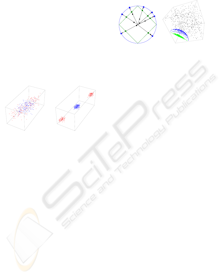
Figure 3: Effect of the normalizer generator in two and

three dimensions. The normalizer ANG maps the posi-

tives (black) onto the unit-L1-sphere to produce the artiﬁ-

cial negatives (internal simplex, green) and then maps them

again into the unit-L2-sphere (external circle, blue) to gen-

erate the normalized positives. This transformation keeps

in-class neighborhood relations and feature correlations be-

tween the two samples. It also generates two close clouds

of points, as it is easy to show that the Euclidean distance

between p

(i)

and a

(i)

is bounded by 1 and likely to be close

to 1. In high dimensions this usually generates interesting

contrasting distributions where the negatives are closer to

negatives and the positives are also closer to the negatives

than to other positives. It is difﬁcult to illustrate this last ef-

fect in two or three dimensions, but it happens consistently,

for example, in the experiments described in section 4.

generated in the four ways explained in the previous

section. We do so over a suite of datasets, for which

it is known that dimensionality reduction is possible

and desirable, in two domains: text classiﬁcation and

functional genomics.

4.1 Experimental Setup

In order to avoid complex experimental setups, we

will consider only reducing to one-dimension through

a linear transformation, represented by e. It is known

that this kind of dramatic dimensionality reduction is

possible for the text classiﬁcation task (Kim et al.,

2005). In this way we avoid the problem of selecting

the optimal dimensionality and the threat of reporting

overoptimistic results due to multiple testing effects.

For the ANG we set the proportion π to 0.5, gener-

ating the same number of artiﬁcial negatives as train-

ing positives. For the left-right ρ parameter we use 20

that always generates well separated clouds of points.

As baseline for dimension reduction techniques we

apply the standard unsupervised LPP (using 5 as the

number of nearest neighbors), PCA and a Gaussian

random projection. Apart from those we also project

over the direction deﬁned by the standard deviation

of each feature, that is, e = (σ

, σ

, . . . , σ

) where σ

is the standard deviation of feature k. The rationale

for this last technique, that we call StdDevPr, will be-

come clear when reading the experiments with text

classiﬁcation. We also report the results got when ap-

plying OCC without dimensionality reduction. The

KDIR 2009 - International Conference on Knowledge Discovery and Information Retrieval

206

following are the two one-class classiﬁers we use:

Gaussian Model (Tax, 2001). Fit a unimodal mul-

tivariate normal distribution to the positives. When

applied to 1-dimensional data, this classiﬁer simply

returns the distance to the mean.

One-class SVM. We use the one-class ν-SVM

(Sch

olkopf et al., 2001) method, that computes hyper-

surfaces enclosing (most of) the positive data. We

set ν, the regularization parameter that controls how

much we expect our training data to be contaminated

with outliers, to 0.05. As it is common practice

in OCC we use the Gaussian kernel, initializing the

width of the kernel to the average pairwise Euclidean

distance in the training set.

In order to select an operating point for the classi-

ﬁers we compute a threshold by assuming that a 5%

of the training data are outliers. This is a common

choice in the one-class literature. The role of thresh-

old selection by train-rejection lies in one or both of

these two assumptions (a) the presence of noise and

some counterexamples in the train data, (b) our clas-

siﬁer is not powerful enough as to accommodate all

positive examples. Another underlying assumption is

that in the training data we have boundary cases, so

that the threshold will not be too tight as for reject-

ing too many positives. A more practical view is that,

probably, this is the most straightforward way of se-

lecting the operating point.

Threshold selection is directly related to the ro-

bustness and capital for one-class classiﬁers general-

ization capabilities. If it is too tight the number of

false negatives will be increased; this can happen if

the noise level speciﬁed by the user is too high. If it is

too loose, the number of false positives will increase;

this will happen if the noise level speciﬁed is too low.

In either case one-class classiﬁers become reject-all

or accept-all machines, which is a very common and

undesirable effect.

For each target class we perform a 10-fold cross-

validation, except for those classes with less than 10

examples, which we ignore, and those with sample

sizes between 10 and 15, for which we perform a

leave-one-out cross validation (in OCC this means

constructing a model using all positives to classify

all negatives, and constructing a model leaving out

each of the positives). Of course, the ANG sampling

and DR computations are also included in the cross-

validation loop, only granting them access to the train

data in each fold. We report the area under the ROC

curve (AUC) and the Balanced Accuracy Rate (BAR)

deﬁned as the average of the True Positive (sensitiv-

ity) and True Negative (speciﬁcity) Rates.

4.2 Text Classiﬁcation

We use a suite of text classiﬁcation problems provided

by Forman (Forman, 2003)

. Those come from sev-

eral well-known text classiﬁcation corpora (ohsumed,

reuters, trec...). In total this accounts for 265 different

classiﬁcation tasks. These are high dimensional (from

2000 to 26832 features) low sample size datasets,

therefore the data is sparse. We use the Bag-of-Words

(BoW) representation that embodies a simplistic as-

sumption of word independence, and normalize each

document to unit-L2 norm, as is usual practice in in-

formation retrieval.

There is a fundamental trap when working with di-

mensionality reduction for text classiﬁcation in OCC.

Due to the sparsity, many of the words do not appear

at all in any of the documents of the class. These

words are unobserved features, features that are con-

stant zero in the training set of a class. Unobserved

features are highly discriminative, but cannot be used

in a principled way for training one-class classiﬁers.

This phenomenon is pervasive, with unobserved ra-

tios per class ranging between 5% and 95% of the fea-

tures in the datasets evaluated. Unobserved features

can make a big difference in performance. For ex-

ample, using the Gaussian classiﬁer the average AUC

varies from 0.9 when allowing unobserved features

in the training set to 0.68 when using only observed

features. In the present experiments we only use ob-

served features.

The results are shown in ﬁgure 4. The baseline

AUC for no dimension reduction is a poor 0.68. Nei-

ther PCA nor LPP provide useful projections when

trained with positive examples only. They are even

harmful performing worse than random projection,

which also performs poorly in this evaluation. In the

ANG realm we realize that both the Uniform and the

Marginal, while still improving over the baseline of

LPP, does not provide the best performance. There-

fore we focus on the three best techniques: Normal-

izer and LeftRight + LPP and the StdDevPr.

The StdDevPr is the best technique in our

test-bench. Its computation is extremely efﬁcient

(O(mn)), requiring only a single pass over the pos-

itive examples. To the best of our knowledge it is

novel and have not been used before, although related

biases can be found in the literature (e.g., the term fre-

quency variance, where in a feature selection context

each word is scored by its variance in the whole cor-

Available for download at http://jmlr.csail.mit.edu/

papers/v3/forman03a.html. We used an extra data-

set, new3s, also supplied by Forman and available

at http://prdownloads.sourceforge.net/weka/19MclassText-

Wc.zip?download

ARTIFICIAL DATA GENERATION FOR ONE-CLASS CLASSIFICATION - A Case Study of Dimensionality Reduction

for Text and Biological Data

207

90.0

100.0

Gauss

60.0

70.0

80.0

100)

ocSVM

20.0

30.0

40.0

50.0

AUC(

0.0

10.0

Marginal Uniform Normalizer LeftRight LPP PCA RandomPr StdDevPr NoDR

SupervisedLPP+ANG NoANG

80 0

90.0

Gauss

60.0

70.0

ocSVM

30.0

40.0

50.0

BAR(x1

0.0

10.0

20.0

Marginal Uniform Normalizer LeftRight LPP PCA RandomPr StdDevPr NoDR

SupervisedLPP+ANG NoANG

Figure 4: Cross-validation AUCs (top) and BARs (bottom)

averaged over 265 datasets/ classes in text classiﬁcation.

pus of positives and negatives (Dhillon et al., 2003)).

It accounts for a very simple rationale: a dimension

(word) is promoted inside a class when it is used a

lot in several of the training documents (modelling

phenomena such as word burstiness (Madsen et al.,

2005)), always in relation to the size of these doc-

uments (recall that we work with normalized docu-

ments).

We came to consider using StdDevPr almost by

accident and only after carefully analyzing the ac-

tual reasons behind the success of LeftRight and the

Normalizer ANGs. We realized that the embeddings

found by LPP using these two ANG techniques where

highly correlated, so it became obvious that LPP was

responding to the same characteristic of our positives

in both cases. It was obvious too that because of the

range-based scaling on the translation part of the Left-

Right ANG, we were artiﬁcially stretching dimen-

sions with high variance. These embeddings are also

highly correlated with those found by StdDevPr, so

the the success when applying these ANGs techniques

is mainly attributed to their similarity to the StdDevPr

technique.

In the bottom part of Figure 4 the performance

of the simple threshold selection technique used is

shown. It is clear that only the StdDevPr enhanced

AUC is well used while both the ranking enhance-

ments provided by LeftRight and Normalizer, in spite

of having the same potential, are lost because of a

poor threshold selection strategy. The target dimen-

sionality (the dimensionality of the data after the ap-

plication of the DR technique) can be regarded as

a regularization parameter (Mosci et al., 2007). In

classiﬁcation, when ﬁxing the thresholding policy, it

controls the trade-off between sensitivity and speci-

ﬁcity; overﬁtting and underﬁtting can be easily pro-

voked by a wrong selection of the target dimension-

ality. Studying the interactions between the threshold

and target dimension selection and the DR and clas-

siﬁcation techniques is essential, but lies beyond the

aims of this paper.

4.3 Translation Initiation Site

Prediction

We applied the same experimental setup to an impor-

tant biological problem: recognizing translation initi-

ation sites (TIS) in a genomic sequence. We used the

dataset described in (Liu and Wong, 2003)

. It has

3312 positive examples and 10063 negatives. These

examples have 927 features that represent counts (rep-

etitions) of k-grams in the DNA sequence. In this

case we do not normalize to unit-L2 norm, but instead

normalize each feature to be in [0, 1] in our training

set. Therefore this time the LeftRight ANG will not

promote high variance directions using the range as a

proxy, since all ranges are the same.

The results are shown in ﬁgure 5. In these results

we see two dominant techniques: using the original

feature set (AUC = 0.82) and the LeftRight + LPP

(AUC=0.92). That accounts for an increase of a 10%

by reducing the dimensionality to 1. Surprisingly,as

shown in the bottom part of the ﬁgure, by using our

simple thresholding technique we get classiﬁcation

accuracies that are competitive with most of the re-

sults in the literature got by using supervised tech-

niques (Liu and Wong, 2003).

We still don’t have conclusive answers for why

LeftRight works so well in this case. Our hypothe-

sis is that our motivation when we designed the sim-

ple LeftRight ANG to collaborate with LPP in order

to “collapse the class” works. Referring to the dis-

tances of the embedded points, LPP does a good job

on getting them very close to zero in the training sets,

and getting similar effects in the test sets. The Uni-

form generator has an analogous effect on the training

sets but the embeddings are not so good at test time

(as reﬂected by its performance in ﬁgure 4), which is

probably due to LPP responding to speciﬁc stochastic

interactions in the artiﬁcial uniform sample.

5 CONCLUSIONS

We have explored the feasibility of artiﬁcial negative

generation techniques in the context of dimensional-

Available for download at http://datam.i2r.a-

star.edu.sg/datasets/krbd/SequenceData/TIS.html

KDIR 2009 - International Conference on Knowledge Discovery and Information Retrieval

208

100.0

Gauss

60.0

70.0

80.0

90.0

00)

ocSVM

20.0

30.0

40.0

50.0

AUC(x

0.0

10.0

Marginal Uniform Normalizer LeftRight LPP PCA RandomPr StdDevPr NoDR

SupervisedLPP+ANG NoANG

100.0

Gauss

70.0

80.0

90.0

)

Gauss

ocSVM

40.0

50.0

60.0

AR(x100

)

10.0

20.0

30.0

0.0

Marginal Uniform Normalizer LeftRight LPP PCA RandomPr StdDevPr NoDR

SidLPP ANG

N ANG

uperv



LPP

+

ANG

o

ANG

Figure 5: Cross-validation AUCs (top) and BARs (bottom)

for the TIS dataset.

ity reduction for one-class classiﬁcation. Applying

very simple artiﬁcial negative generation techniques

working together with a locality preserving dimen-

sion reduction has shown promising results in a ex-

periment with a comprehensive set of text classiﬁca-

tion datasets and a genomics dataset. This area of re-

search is by its very nature speculative, as ultimately

one always needs to rely on the relations between the

artiﬁcial sample and the actual negatives, the latter be-

ing unknown. It is also the case that for each ANG

mechanism we can ﬁnd the corresponding unsuper-

vised bias. In the case of text classiﬁcation we found

via this indirect approach that stretching up the di-

rections - words - which account for more variance

within the class once the documents are normalized

is a fast, reliable and class-dependent bias for dimen-

sion reduction in one-class classiﬁcation. For the ge-

nomics dataset one of our proposed techniques excels

at ﬁnding discriminative representations and all seems

to indicate that this is due to our algorithm-design ra-

tionale working as expected.

This work can be extended by studying synergies

between ANG and corresponding supervised tech-

niques. For example, for text classiﬁcation, apply-

ing Linear Discriminant Analysis together with para-

metric ANG techniques has shown consistent good

performance. We are also exploring the potential to

incorporate the other bit of information we have in

OCC, the testing point, to guide the creation of our ar-

tiﬁcial negatives. Artiﬁcial negatives could also lead

to data-driven techniques for other tasks in the clas-

siﬁcation system, like the threshold or target dimen-

sionality selections.

REFERENCES

Abe, N., Zadrozny, B., and Langford, J. (2006). Outlier

detection by active learning. In KDD: International

Conference on Knowledge Discovery and Data Min-

ing, pages 767–772.

Breiman, L. (2001). Random forests. Machine Learning,

45(1):5–32.

Chapelle, O., Sch

olkopf, B., and Zien, A., editors (2006).

Semi-Supervised Learning. The MIT Press, Cam-

bridge, MA.

Chung, F. R. K. (1997). Spectral Graph Theory (CBMS

Regional Conference Series in Mathematics, No. 92).

American Mathematical Society.

Dhillon, I., Kogan, J., and Nicholas, C. (2003). Feature se-

lection and document clustering. In A Comprehensive

Survey of Text Mining, pages 73–100. Springer.

El-Yaniv, R. and Nisenson, M. (2006). Optimal single-class

classiﬁcation strategies. In NIPS: Advances in Neural

Information Processing Systems.

Fan, W., Miller, M., Stolfo, S., Lee, W., and Chan, P.

(2004). Using artiﬁcial anomalies to detect unknown

and known network intrusions. Knowledge and Infor-

mation Systems, 6(5):507–527.

Forman, G. (2003). An extensive empirical study of fea-

ture selection metrics for text classiﬁcation. Journal

of Machine Learning Research, 3:1289–1305.

Franc¸ois, D. (2008). High-dimensional Data Analysis:

From Optimal Metrics to Feature Selection. VDM

Verlag.

Francois, D., Wertz, V., and Verleysen, M. (2007). The

concentration of fractional distances. IEEE Trans. on

Knowl. and Data Eng., 19(7):873–886.

Hastie, T., Tibshirani, R., and Friedman, J. H. (2001). The

Elements of Statistical Learning. Springer.

He, X. and Niyogi, P. (2003). Locality preserving projec-

tions. In NIPS: Advances in Neural Information Pro-

cessing Systems.

Hempstalk, K., Frank, E., and Witten, I. H. (2008). One-

class classiﬁcation by combining density and class

probability estimation. In ECML: European Confer-

ence of Machine Learning.

Kim, H., Howland, P., and Park, H. (2005). Dimension re-

duction in text classiﬁcation with support vector ma-

chines. Journal of Machine Learning Research, 6:37–

53.

Liu, H. and Wong, L. (2003). Data mining tools for biolog-

ical sequences. Journal of Bioinformatics and Com-

putational Biology, 1(1):139–167.

Madsen, R. E., Kauchak, D., and Elkan, C. (2005). Model-

ing word burstiness using the dirichlet distribution. In

ICML: International Conference on Machine Learn-

ing, pages 545–552.

Manevitz, L. M. and Yousef, M. (2001). One-class SVMs

for document classiﬁcation. Journal of Machine

Learning Research, 2:139–154.

ARTIFICIAL DATA GENERATION FOR ONE-CLASS CLASSIFICATION - A Case Study of Dimensionality Reduction

for Text and Biological Data

209

Mosci, S., Rosasco, L., and Verri, A. (2007). Dimension-

ality reduction and generalization. In ICML: Interna-

tional Conference on Machine Learning, pages 657–

664.

Sch

olkopf, B., Platt, J. C., Shawe-Taylor, J. C., Smola, A. J.,

and Williamson, R. C. (2001). Estimating the support

of a high-dimensional distribution. Neural Computa-

tion, 13(7):1443–1471.

Scott, C. and Blanchard, G. (2009). Novelty detection: Un-

labeled data deﬁnitely help. In AISTATS: Artiﬁcial In-

telligence and Statistics, JMLR: W&CP 5.

Scott, C. D. and Nowak, R. D. (2006). Learning minimum

volume sets. Journal of Machine Learning Research,

7:665–704.

Shi, T. and Horvath, S. (2006). Unsupervised learning with

random forest predictors. Journal of Computational

& Graphical Statistics, 15:118–138.

Steinwart, I., Hush, D., and Scovel, C. (2005). A classiﬁ-

cation framework for anomaly detection. Journal of

Machine Learning Research, 6:211–232.

Tax, D. M. J. (2001). One-class classiﬁcation. Concept

learning in the absence of counterexamples. PhD the-

sis, Delft University of Technology.

Tax, D. M. J. and Duin, R. P. W. (2002). Uniform object

generation for optimizing one-class classiﬁers. Jour-

nal of Machine Learning Research, 2:155–173.

Tax, D. M. J. and Muller, K.-R. (2003). Feature extrac-

tion for one-class classiﬁcation. In ICANN/ICONIP:

Joint International Conference on Artiﬁcial Neural

Networks and Neural Information Processing.

Villalba, S. D. and Cunningham, P. (2007). An evaluation of

dimension reduction techniques for one-class classiﬁ-

cation. Artiﬁcial Intelligence Review, 27(4):273–294.

KDIR 2009 - International Conference on Knowledge Discovery and Information Retrieval

210