CLASSICATION BY SUCCESSIVE NEIGHBORHOOD
David Grosser, Henri Ralambondrainy and Noel Conruyt
Laboratoire d’Informatique et Math
´
ematiques, Universit
´
e de la R
´
eunion, 97490 Sainte-Clotilde, France
Keywords:
Classification, Similarity, Nearest neighbors, Structured data, Systematics.
Abstract:
Formalization of scientific knowledge in life sciences by experts in biology or Systematics produces arbores-
cent representations whose values could be present, absent or unknown. To improve the robustness of the
classification process of those complex objects, often partially described, we propose a new classification
method which is iterative, interactive and semi-directed. It combines inductive techniques for the choice of
discriminating variables and search for nearest neighbors based on various similarity measures which take into
account structures and values of the objects for the neighborhood computation.
1 INTRODUCTION
Systematics is the scientific discipline that deals with
listing, describing, naming, classifying and identify-
ing living beings. In the frame of environmental sci-
ences, the acquisition and production of knowledge
on biological specimens and taxa is an essential part
of the work of systematicians (Winston, 1999). In-
deed, being able to describe, classify and identify a
specimen from morphological characters is a first step
for monitoring biodiversity because it gives access
to information relative to its species name (Biology,
Geography, Ecology, etc.). This process can be as-
sisted with computer science decision support tools.
In return, such complex domains deliver interesting
symbolical and numerical knowledge representation
and processing problems to the knowledge engineer-
ing and computer science community.
Indeed, classical discrimination methods devel-
oped in the frame of data analysis or machine learn-
ing, such as classification or decision trees (Breiman
et al., 1984), (Quinlan, 1986) or more recent methods
developed in the data mining field such as association
rules mining (Piatetsky-Shapiro, 1991) or Multifactor
dimensionality reduction (Zhu and Davidson, 2007)
are not sufficient, because they do not cope with re-
lations between attributes, missing data, and are not
very tolerant to errors in descriptions.
The considered problem that we are faced with is
to determine the class of a structured description that
is partially answered and, eventually contains errors,
from a referenced case base, this last one be a priori
classified by qualified experts in k-classes. The pro-
posed discrimination method proceeds by inference
of successive neighboring. It is inductive, interac-
tive, iterative and semi-directed. It combines induc-
tive techniques of discriminatory variables and neigh-
bors search, with the help of a similarity measure that
takes into account the structure (dependencies of vari-
ables) and the content (missing and unknown values).
2 DATA REPRESENTATION
Within a knowledge base, observations are described
with the help of descriptive models. A descriptive
model represent an ontological knowledge about the
considered domain and contains descriptors structure
and organization.
2.1 The Descriptive Model
The descriptive model (fig. 1), or schema, is a
rooted tree M = (A, U), where A is a set of
nodes(attributes), and U a set of edges. Leaves
are single classical attributes, as numerical or nomi-
nal ones, called ”basic attributes”. Nodes are ”struc-
tured attributes”, sub-trees made of several attributes.
For example, A
j
:< A
1
, . . . , A
p
> denotes a structured
attribute where A
j
is the root of the sub-tree and
A
1
, . . . , A
p
, are the sons, structured or basic attributes,
the components of A
j
.
288
Grosser D., Ralambondrainy H. and Conruyt N. (2009).
CLASSIFICATION BY SUCCESSIVE NEIGHBORHOOD.
In Proceedings of the International Conference on Knowledge Discovery and Information Retrieval, pages 288-291
DOI: 10.5220/0002299002880291
Copyright
c
 SciTePress

Figure 1: This example shows a description part of a speci-
men belonging to the genus Stylocoeniella.
2.2 Object Representation
An object, described by a schema M , is a tree de-
rived from M where each basic attribute has been
valued (fig. 1). A skeleton represents the structure
of an object, it describes the state of each compo-
nent: present (+), absent (or missing) (-), or unknown
(∗). We denote by S = {+, −, ∗}. A map σ : A → S
defines a labeled rooted tree H
σ
= (A
σ
, U) where
A
σ
= {(A
j
, σ(A
j
))|A
j
∈ A }. The skeleton of an object
is represented by H
σ
. The nodes of a skeleton must re-
spect the following consistency constraints: for each
structured attribute B :< B
l
>
l∈L
, we must have:
1. “The sons of a missing node must be missing”: if
σ(B) = − then σ(B
l
) = −, for l ∈ L,
2. “The sons of an unknown node are unknown or
missing”: if σ(B) = ∗ then σ(B
l
) = ∗|−, for l ∈ L.
3. “The sons of a present node may be present, miss-
ing or unknown”: if σ(B) = + then σ(B
l
) =
+| − |∗, for l ∈ L.
We denote by H the set of skeletons that are
consistent. Assume that is given a set of basic at-
tributes names A
q
and corresponding domains D
q
for
q ∈ Q. For any object, a basic attribute A
q
is valued
in D
q
only If the attribute is present. Missing val-
ues will be denoted by ⊥ and unknown values by ∗,
then Γ
q
= D
q
∪ {⊥} ∪ {∗}} is the new domain for a
basic attribute A
q
. The set of values of an object o
is v
o
= (v
q
)
q∈Q
where v
q
∈ Γ
q
. Let Γ
Q
= u
q∈Q
Γ
q
,
an object is described with its skeleton and values :
o = (H
σ
o
, v
o
) ∈ E = H × Γ.
3 SIMILARITY MEASURES
In this section, we propose a function to evaluate
the similarity level between a pair of skeletons. The
weight m(A
j
) of the attribute A
j
is the number of at-
tributes which is made of. It means that the contribu-
tion of a structured attribute in the similarity evalua-
tion of skeletons depends on the number of its com-
ponents. Given a comparison map λ : S × S −→ [0, 1]
(table 1), the structural weighted similarity measure,
between the skeletons H
σ
1
et H
σ
2
, is defined as:
ζ
SW
(H
σ
1
, H
σ
2
) =
Σ
j∈J
m(A
j
)λ({σ
1
(A
j
), σ
2
(A
j
)})
Σ
j∈J
m(A
j
)
.
If we take α
1
j
= β
1
j
= α
2
j
= γ
j
= β
2
j
= 0 (table 1) and a
weight equal to 1 for all attributes, then the proposed
function is the well-known Sokal index (Sneath and
Sokal, 1973). Another possible choice is to take β
1
j
=
β
2
j
= γ
j
= 0 for the comparison of unknown values
and define λ({σ
1
(A
j
) = +, σ
2
(A
j
) = −}) = α
1
j
as the
ratio of missing sons of A
j
in the skeleton H
σ
1
.
Table 1: Values of a comparaison map λ for a given node
A
j
.
H
σ
1
H
σ
2
+ − ∗
+ 1 α
1
j
β
1
j
− α
2
j
1 γ
j
∗ β
2
j
γ
j
1
For some applications, users wish emphasize
present rather than missing or unknown attributes.
For that purpose, we define the structural recursive
similarity measure built from a map λ
r
as follow:
if A
j
is a basic attribute, presents both in H
σ
1
and
H
σ
2
: σ
1
(A
j
) = σ
2
(A
j
) = + then:
λ
r
(+, +) = 1, (1)
else A
j
:< A
l
>
l∈L
is a structured attribute and
λ
r
(+, +) =
1 + Σ
l
m(A
l
)λ
r
({σ
1
(A
l
), σ
2
(A
l
)})
m(A
j
)
(2)
This similarity measure is recursively computed from
the root A:
ζ
SR
(H
σ
1
, H
σ
2
) = λ
r
({σ
1
(A), σ
2
(A)}) (3)
4 CLASSIFICATION BY
SUCCESSIVE
NEIGHBORHOOD
The proposed classification method allows to deter-
mine the membership of an individual to a particular
class which is partially described by a user and com-
prising eventually some errors. It takes into account
CLASSIFICATION BY SUCCESSIVE NEIGHBORHOOD
289

dependences relations between attributes. The prin-
ciple consists with to select a neighborhood V , i.e. a
descriptions set (individuals or classes) close to cur-
rent description with the help of the similarity mea-
sure. A set of candidates classes is computed from
the neighbor set. The method seeks then to supple-
ment the missing information, firstly with the appli-
cation of coherency rules, secondly by proposing a
set of discriminants attributes. A new neighborhood
is then computed on the basis of the new partial de-
scription. The process is reiterates until obtaining a
homogeneous descriptions set.
4.1 Neighborhood Classification
Algorithm
The iterative process to predict the class of a speci-
men, from a given description e, is made of the fol-
lowing steps:
1. Initialize radius value ∆ to the max of the distance
of e to the set of observations.
2. Determine the set of objects inside of the sphere
of radius ∆ centered at e,
3. Compute the classification scores of the a priori
classes,
4. Compute a new radius value ∆ from the set of
neighbors,
5. Repeat 2, 3, 4 until stopping condition is satisfied
4.1.1 Neighbors Set
The neighbors of e at iteration m is the set of objects
inside of the sphere of radius ∆
m
centered at e:
N
(m)
= {o ∈ O | d(e, o) < ∆
m
}.
The radius value is determined from the maximum
distance, a dissimilarity measure between e and a set
A :
D
max
(e, A) = max
a∈A
d(e, a)
then ∆
m
is written: ∆
m
= D
max
(e, N
(m−1)
). It is easy to
show that {∆
m
} is a decreasing sequence. If each ob-
ject o
i
has a normalized weight p
i
, then the dispersion
distance:
D
disp
(e, A) = Σ
o
i
∈A
p
i
d
2
(e, o
i
)
is suitable, we can show that {∆
m
= D
disp
(e, N
(m−1)
)}
is still a decreasing sequence.
4.1.2 Class Classification Score
The examples O are pre-classified into classes de-
noted by {C
l
}
l∈K
. Let Pr(C
l
|N
(m)
) =
|C
l
∩N
(m)
|
|N
(m)
|
be the
probability of the cluster C
l
given the set of neighbors
N
(m)
or the relative frequency of the cluster C
l
in the
set of neighbors N
(m)
. The label that should be as-
signed to input e will be chosen from clusters such
as its probability Pr(C
l
|N
m
) are significantly different
from the prior probability of the cluster Pr(C
l
|O) =
|C
l
|
|0|
. Usual significant statistical test of frequencies
may be used or defined user threshold for this pur-
pose. Then, the classification score of the class C
l
at
iteration m is
R
l
=
Pr(C
l
|N
m
)
Pr(C
l
|O)
.
4.1.3 Stopping Condition
The initial value of the radius is ∆
0
= D
max
(e, O).
As the sequence of radius is decreasing, then the se-
quence of the set of neighbors {N
(m)
} is also decreas-
ing. The iterative process is suspended, when the
maximum of a classification score R
l
of a class C
l
is
greater than a threshold r
0
> 1. In practice r
0
= 2, the
class with the best score is proposed to the user as the
label of the specimen. Otherwise, a minimum size of
the neighbors set (ten percent of the population size
for example) is used as a stopping criteria. We can
notice that it is more easier to the user to fix the previ-
ous thresholds than to give a good number k of nearest
neighbors.
4.1.4 Discriminant Attributes Selection
An ordered list of informative variables is computed
at each iteration of the classification process. The first
element is exposed as a question to the user who can
choose an alternative variable from the list or an un-
known answer. The list is built in function of several
criteria:
1. Attribute potentiality. The method considers only
at each step the attributes which can be indicated,
i.e., those for which there exists a components
(nodes) chain whose presence is proven.
2. Discriminant power. Choice of different classi-
cal criteria computing the information gain used
in machine learning such as Shannon entropy or
Gini index.
3. Background knowledge by using attributes
weighting in the descriptive model.
KDIR 2009 - International Conference on Knowledge Discovery and Information Retrieval
290

5 ILLUSTRATIVE EXAMPLE
The famous Anderson’s Iris data is used to illustrate
the neighborhood classification algorithm. This data
set contains 150 plants from 3 specific species charac-
terized by 4 attributes. The task is to predict the class
of a given specimen, its description e is a slight mod-
ification of a plant description of a setoza specy (see
Table 2).
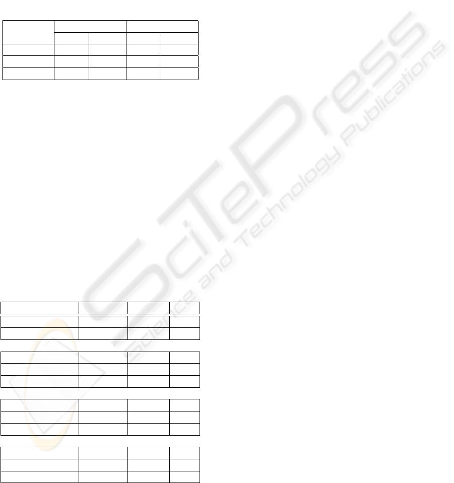
Table 2: Specimen.
Attribute petal sepal
Specimen width length width length
e
1
- 3.1 - -
e
2
- 3.1 - 2.19
e 7 3.1 5.97 2.19
To test the performance of the algorithm, we start
to identify the given specimen, using only the petal
length value, the other values are considered as ”un-
known” (specimen e
1
in Table 2). After 16 iterations
(Table 3), the algorithm stops as the size of neighbors
is less than 15 (the threshold has been fixed to be ten
percent of the population size). Scores of the 3 classes
are not satisfactory as they are lower than 2. The at-
tribute sepal length is proposed to be assigned a value,
according to its discriminatory ability. The algorithm
is applied to the resulted specimen e
2
. After 46 itera-
tions, the class setoza has the best score greater than 2,
and is proposed to be the specimen label. In contrast
to decision tree methods, we can notice that the identi-
fication process can be performed with attributes that
have not necessarily a good discriminatory ability.
Table 3: Experiments.
Cluster versicolor virginica setoza
Size Cluster (C) 50 50 50
Pr(C|O) 33.3 33.3 33.3
Identification of e
1
: versicolor ? (iteration =16)
Size Neighbor (N) 5 3 4
Pr(C|N) 41.7 25 33.3
Cluster score R 1.25 0.75 1
Identification of e
2
: setoza (iteration =46)
Size Neighbor 0 21 48
Pr(C|N) 0 30.4 69.6
Cluster score R 0 0.91 2.08
Identification of e: setoza (iteration =66)
Size Neighbor 0 24 49
Pr(C|N) 0 32.9 67.1
Cluster score R 0 0.99 2.01
6 CONCLUSIONS AND
PERSPECTIVES
To identify a biological object and to associate a taxon
to it, most of the time systematicians proceed in two
phases. The synthetic phase, by global observation
of the most visible characters reduces the field of in-
vestigation. The analytical phase, by precise observa-
tion of discriminating attributes refines research until
obtaining the result. The classification by successive
neighborhood from a partial description that we pro-
pose presents the interest to correspond to the reason-
ing followed by biologists. Starting from a partial de-
scription generally containing the most visible or easy
to observe and describe attributes, the method sug-
gests relevant information necessary to supplement to
determine the most probable class. Moreover, it is
error tolerant because an erroneous information can
nevertheless lead to a satisfactory result due to the
fact that a smooth matching is carried using similarity
function out on filled values rather than a strict one.
We expect that the method is generic and applica-
ble on any fields where structured or semi-structured
data are considered, such as XML data format, RDF
graph structures or OWL Ontologies. It’s enough to
lay out an operator of generalization and a similarity
index adapted to the considered data. This method
is in evaluation progress on the ” knowledge base on
corals of the Mascareignes archipelago” which counts
approximately 150 taxa and 800 complex descrip-
tions.
REFERENCES
Breiman, L., Freidman, J. H., Olshen, R. A., and Stone,
C. J. (1984). Classification and regression trees.
Wadsworth, Belmont.
Piatetsky-Shapiro, G. (1991). Discovery, analysis, and pre-
sentation of strong rules. Knowledge Discovery in
Databases, AAAI/MIT Press, Cambridge, MA.
Quinlan, J. (1986). Induction of decision trees. Machine
Learning, 1:81–106.
Sneath, H. and Sokal, R. (1973). Numerical Taxonomy.
W.H. Freeman.
Winston, J. E. (1999). Describing Species: Practical Taxo-
nomic Procedure for Biologists. New York: Columbia
University Press.
Zhu, X. and Davidson, I. (2007). Knowledge Discovery
and Data Mining: Challenges and Realities with Real
World Data. Idea Group Inc.
CLASSIFICATION BY SUCCESSIVE NEIGHBORHOOD
291