
COMPARISON BETWEEN SVM AND ANN FOR MODELING
THE CEREBRAL AUTOREGULATION BLOOD FLOW SYSTEM
Max Chacón, Claudio Araya, Marcela Muñoz
Departamento de Ing. Informática, Universidad de Santiago de Chile, Av. Ecuador 3659, Santiago, Chile
Ronney B. Panerai
University of Leicester, Departments of Cardiovascular Sciences, LE1 5WW, Leicester, U.K.
Keywords: Support vector machine, Artificial neural networks, Cerebral blood flow autoregulation.
Abstract: The performance of SVMs and ANNs as identifiers of time systems is compared with the purpose of
analyzing the Cerebral blood flow Autoregulation System, one of the main systems in the field of cerebral
hemodynamics. The main variables of this system are Arterial Blood Pressure (ABP) variations and changes
in End-tidal pCO
2
(EtCO
2
). In this work we show that models that have ABP and EtCO
2
as input, trained
with the SVM, are superior to ANN models in terms of the fit of an unknown set, and they are also more
adequate for measuring the influence of EtCO
2
on Cerebral Blood Flow Velocity.
1 INTRODUCTION
Since the introduction of SVMs in the early 1990s,
they have been applied to a large number of
classification or regression problems, but little work
has been done on their use as predictors of temporal
series or for identifying systems over time. Among
the work that has centered on their application over
time, the proposals of J. Suykens’ group stand out
(Suykens et al., 2000; Espinoza et al., 2007) in the
development of LS-SVM, and that of A. Martínez
and J.L. Rojo (Rojo-Alvarez et al., 2004; Martínez-
Ramón et al., 2006). But these works are centered
mainly on forecasting known chaotic series that are
used as “benchmarks” of the proposed methods.
In the field of biological signals the use of SVMs
has been focused on applications in which the
signals’ characteristics are extracted from the signals
to use them as static classifiers (Acir and Guzelis,
2004).
In this paper we apply SVMs (as multivariate
identifiers of systems over time) to one of the main
problems of cerebral hemodynamics: identification
of the Cerebral Blood Flow Autoregulation System
(CAS). This method is also compared with the
performance of Artificial Neural Networks (ANNs).
The main mechanisms that affect the CAS are
autorregulation of Arterial Blood Presure (ABP) and
the reactivity of cerebral blood vessels to arterial
CO
2
pressure (EtCO
2
) (Widder et al, 1986).
The most common technique for determining
reactivity of a subject’s blood vessels to CO
2
is to
measure the change that occurs in CBF as a
consequence of breathing a mixture of air and 5%
CO
2
(Panerai et al., 2000), using the measurements
made with the Transcranial Doppler Ultrason to
estimate CBF Velocity (CBFV).
The works of Panerai and Simpson (Panerai et
al., 2000; Simpson et al., 2000) has modeled both
the EtCO
2
signal and Median Arterial Blood
Pressure (MABP) to predict CBFV, using linear
models such as cross-correlation analysis over
frequency and auto-regressive models over time.
These models have shown that under baseline
conditions (spontaneous fluctuations)
CO
2
accounts
for part of the variability of CBFV, and when
changes in CO
2
are introduced it is possible to
represent the relation with CBFV by means of a
linear model.
The only report on the use of a data-based
nonlinear model to study the MABP and EtCO
2
variables is that of Mitsis et al. (2004), who use a
special Laguerre-Volterra network to analyze the
baseline MABP and EtCO
2
signals of ten subjects.
The conclusions show that the relation between
EtCO
2
and CBFV are highly nonlinear at low
522
Chacón M., Araya C., Muñoz M. and B. Panerai R. (2009).
COMPARISON BETWEEN SVM AND ANN FOR MODELING THE CEREBRAL AUTOREGULATION BLOOD FLOW SYSTEM.
In Proceedings of the International Joint Conference on Computational Intelligence, pages 522-525
DOI: 10.5220/0002279205220525
Copyright
c
SciTePress

frequencies and the time varying system. That paper
is centered mainly on the analysis of frequency, it
uses a network based on polynomials that
approximate efficiently only up to the third order,
and the CO
2
signal considers only the baseline state.
In the present paper we use more general tools
(SVM and ANN), that allow modeling MABP and
CO
2
as input, with CBFV as output for the baseline
case and for induced 5% CO
2
changes. With these
elements we will evaluate the nonlinear behavior of
the SVM and its comparison with ANNs from the
standpoint of numerical precision, to predict a
previously unknown CBFV signal, and we will
subject the models to CO
2
changes to evaluate their
ability as a clinical method for obtaining reactivity
to CO
2
.
2 METHOD AND MATERIALS
2.1 Subjects and Measurements
The data used in this work were obtained from 16
voluntary subjects (aged between 25 and 51 years)
who had no history of vascular diseases or
neurological problems.
The study was approved by the ethics committee
of the Royal Infirmary of Leicester, UK.
CBFV was measured in cm/s in the medial
cerebral artery by means of a Scimed QVL-120
Doppler Transcranial system with a 2 MHz
transducer. MABP was measured in mmHg on the
patient’s finger with a noninvasive Finapres 2300
Ohmeda monitor. EtCO
2
levels were recorded on a
Datex Normocap 200 infrared capnograph connected
to the subject through a nasal mask.
The three signals were filtered with an order 8
low pass Butterworth filter with a 20-Hz cutoff
frequency. The signals were then interpolated
linearly and normalized between 1 and -1.
The most common technique for carrying out the
test of reactivity to CO
2
(standard reactivity) is to
breathe a mixture of air and CO
2
and determine the
changes that it causes in the CBFV. In this work
each subject was first allowed to breathe a sample of
ambient air for 5 minutes and was then made to
breathe a mixture of air and 5% CO
2
for
approximately 3 minutes.
2.2 Support Vector Machine
The SVM algorithm adopted was the ν-SVM,
introduced by Schölkopf et al. (1998). It is based on
the statistical theory of learning which introduced
regression as the fitting of a tube of radius ε to the
data. The decision boundary for determining the
radius of the tube is given by a small subset of
training examples called Support Vectors (SV).
Assuming
x
G
represents the input data vector, the
output value
)(xf
G
is given by the SVM regression
using a weight vector
w
G
.
bxwxf
+
=
• )()(
G
G
G
,
, ,, RR ∈∈ bxw
N
G
G
(1)
where b is a constant obtained from
w
G
.
The variation of the ν-SVM introduced by
Schölkopf et al. (1998) consists in adding ε to the
minimization problem, weighted by a variable
ν
that
adjusts the contribution of
ε
between 0 and 1.
minimize
⎟
⎟
⎠
⎞
⎜
⎜
⎝
⎛
++=
∑
=
l
i
i
lCww
1
2
1
),(
ξνεξθ
GG
(2)
In the above equation, l represents the total
dimension of the data (number of cases), C is a
model parameter determining the trade-off between
the complexity of the model, expressed by
w
G
, and
the points that remain outside the tube. Slack
variables
ξ
depend on the distance of the data points
from the regression line.
We used ε-insensitive loss function.
The solution of this minimization problem for
obtaining the weight vectors
w
G
is found by the
standard optimization procedure for a problem with
inequality restrictions when applying the conditions
of Kuhn-Tuker to the dual problem. The main
advantage of introducing parameter ν ∈ [0-1] is to
make it possible to control the error fraction and the
number (or fraction) of SVs with only one
normalized parameter.
To solve a nonlinear regression problem it is
sufficient to substitute the inner product between
two independent original variables
ji
xx
GG
•
(Eq. 1) by
a kernel function gaussian radial base function
(RBF),
))2/(exp(),(
2
2
σ
jiji
xxxxk
G
G
G
G
−−= (3)
2.3 Artificial Neural Networks
Use was made of static neural networks with
external recurrence, which correspond to the
structure of a multilayer perceptron that can be
trained using the classic Backpropagation algorithm.
Different learning algorithms were evaluated,
such as One Step Secant, Delta Bar Delta,
COMPARISON BETWEEN SVM AND ANN FOR MODELING THE CEREBRAL AUTOREGULATION BLOOD
FLOW SYSTEM
523
Backpropagation through time, and Levenberg
Marquardt, with the latter delivering the best results.
This mixed algorithm combines a descending
gradient with one of quasi-Newton type. Eq. 4
shows how the algorithm updates the weight at each
iteration.
[]
eJIJJ
TT
kk
1
1
−
+
+−=
μωω
(4)
where
1+k
ω
is the weight vector in iteration k+1,
k
ω
is the weight vector in iteration k, J is the first
derivatives Jacobian matrix, and e corresponds to the
network error vector. Factor
μ
is reduced at each
successful step, controlling the trade off between a
descending gradient and a quasi-Newton method.
Early Stopping was used to get a good
generalization in the set of tests (Demuth and Beale,
2001).
To implement recurrence in both the SVMs and
the ANNs we used external feedback of the delayed
outputs (v(t)=CBFV), and current inputs
(p(t)=MABP, c(t)=EtCO
2
) and past time instants are
considered. Training is carried out estimating a
forward step, as shown in Eq. 5 .
))(),...,(),...,(
),...,(),(),...,1(()(
ˆ
cp
v
ntctcntp
tpntvtvftv
−−
−−=
(5)
The prediction is obtained using the estimated
values, as shown in Eq. 6.
))(),...,(),...,(
),...,(),(
ˆ
),...,1(
ˆ
()(
ˆ
cp
v
ntctcntp
tpntvtvftv
−−
−−=
(6)
2.4 Evaluation and Statistics
To evaluate the learning of the models (training and
evaluation) use is made of the correlation between
the model’s response (
v
ˆ
) and the real output signal
(v).
To analyze the physiological behavior the
responses to an MABP step and an EtCO
2
step are
examined in terms of their dynamics. To evaluate
the clinical potential of the models the reactivity
index is obtained, extracted from the models after
applying to them a CO
2
step, and it is compared with
the calculation of the standard reactivity test, which
is obtained when the subject inhales 5% CO
2
.
The statistical significance was evaluated using
Wilcoxon’s paired test considering that there are
differences if p<0.05.
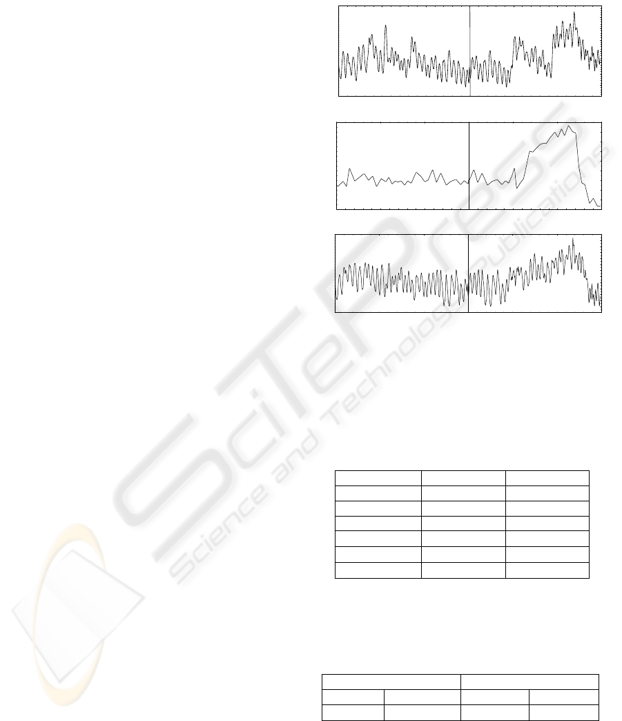
3 RESULTS
Figure 1 shows the three signals after pre-processing
them.
0 100 200 300 400 500 600
Time (s)
90
95
100
105
110
115
120
125
130
ABP (mmHg)
0 100 200 300 400 500 600
Time (s)
5,4
5,6
5,8
6,0
6,2
6,4
6,6
6,8
7,0
7,2
EtCO
2
(%)
0 100 200 300 400 500 600
Time (s)
36
38
40
42
44
46
48
50
52
54
56
58
60
62
CBFV (cm/s)
Figure 1: Representative time-series of MABP, EtCO
2
,
and CBFV showing spontaneous fluctuations during
baseline (left) and breathing of 5% CO
2
in air (right).
The averages and modes of the best parameters
for the 16 SVM models are shown in Table 1.
Table 1: Model parameters for SVM structures tested.
Parameters Baseline 5% CO
2
n
p
4 [4-8] 5 [3-6]
n
v
3 [1-3] 1 [1-3]
n
c
3 [2-4] 2 [2-4]
C
395.0
±
404.4 343.1
±
416.6
ν
0.32
±
0.28 0.43
±
0.30
σ
3.72
±
4.98 19.75
±
13.24
The modes of the parameters for the ANNs are
equal for the baseline and the 5% CO
2
cases, with
n
p
=n
c
=n
v
=2 and 8 neurons in the hidden layer.
Table 2: Correlations of the models for the set of tests.
SVM ANN
Baseline 5% CO
2
Baseline 5% CO
2
0.76
±
0.1 0.95
±
0.03 0.77±0.16 0.82±0.11
The results of the correlations in the set of tests
appear in Table 2. In the baseline case it is seen that
there are no significant differences between SVM
and ANN (p=0.71), but when compared with the
IJCCI 2009 - International Joint Conference on Computational Intelligence
524

changes in CO
2
, the test shows that the SVMs are
significantly better than the ANNs (p=0.0004).
The reactivity curves for both types of models
show an acceptable physiological response, with
those obtained from training with changes in 5%
CO
2
always better.
The average results of the standard reactivity test
of the 16 subjects was 4.05±1.38%/mmHg,
(average±SD).
Entering a normalized step response between [0-
1] into the EtCO
2
input it is possible to measure each
subject’s reactivity. The average values of each
model are shown in Table 3.
Table 3: Reactivity of the models (%/mmHg).
SVM ANN
Baseline 5% CO
2
Baseline 5% CO
2
4.32 ±4.2 4.44 ±1.9 2.22 ±3.0 3.13
±
1.4
When conducting a hypothesis test between the
standard reactivity test and the reactivities obtained
by the models, it is seen that there are no differences
with the reactivities extracted from the SVMs in
both cases. Compared to ANNs, the test is
significantly different in the baseline case (p=0.002)
and has values very close to the limit for CO
2
changes (p=0.07)
4 CONCLUSIONS
The results not only show the superiority of SVMs
in terms of precision and calculation of reactivity,
but it is also seen that they show a smaller variance,
particularly in the case of CO
2
changes.
The baseline mean square error of the SVM
model is 3%, which is much better than the 20%
reached in the work of Mitsis et al. (2004).
We believe that both the global optimization and
the slack-variable properties of SVMs are
responsible for the better results in comparison with
the Artificial Neural Networks.
The main future challenges involve new studies
in the field of biomedical signals that may allow the
evaluation of the other properties of the SVM, such
as the ability to represent time varying phenomena.
ACKNOWLEDGEMENTS
This work was supported by a research grant from
FONDECYT, Government of Chile, Project
1070070.
REFERENCES
Acir, N., and Guzelis, C., 2004, Automatic spike detection
in EEG by a two-stage procedure based on support
vector machines. Comput Biol Med. Vol. 7, 561-75.
Demuth, H., Beale. M., 2001, Neural network toolbox
user’s guide, The MathWorks Inc.
Espinoza, M., Suykens, J.K.A., Belmans, R., and De
Moor, B., 2007, Electric load forecasting - using
kernel based modeling for nonlinear system
identification,” IEEE Control Systems Magazine
(Special Issue on Applications of System
Identification), 43-57.
Martínez-Ramón, M., Rojo-Álvarez, JL., Camps-Valls, G.
Navia-Vázquez, A., Soria-Olivas, E., and Figueiras-
Vidal, A., 2006, Support vector machines for
nonlinear kernel ARMA system identification, IEEE
Trans. on Neural Net., Vol. 17, 1617-1622.
Mitsis, G., Poulin, M., Robbins, P., Marmarelis, V., 2004,
Nonlinear modeling of dinamic effects of arterial
pressure and CO
2
variations on cerebral blood flow in
healthy humans, IEEE Trans. Biomed. Eng., Vol. 51,
1932-1943.
Panerai, R., Simpson, D., Deverson, S., Mahony, P.,
Hayes, P., Evans, D., 2000, Multivariate Dynamic
Analysis of Cerebral Blood Flow Regulation in
Humans”, IEEE Trans. Biomed. Eng., Vol 47, 419-
423.
Rojo-Álvarez, JL, Martínez-Ramón, M. Prado-Cumplido,
M Artés-Rodríguez, Figueiras-Vidal, A., 2004,
Support Vector Method for Robust ARMA System
Identification, IEEE Tran. Signal Process. Vol. 52,
155-164.
Simpson, D., Panerai, R., Evans, D., Garnham, J., Naylor,
A., Bell, P., 2000, Estimating normal and pathological
dynamic responses in cerebral blood flow velocity to
step changes in end-tidal pCO
2
, Med. Biol. Eng.
Comp., Vol. 38, 535-539.
Schölkopf, B., Smola, A., Williamson R.C., and Bartlett,
P.L., 1998, New support vector algorithms, Neural
Computation, Vol. 12, 1083-1121,.
Suykens, JAK., Vandewalle J., 2000, Recurrent least
squares support vector machines, IEEE Trans. on
Circuits and Systems I, Vol. 47, 1109–1114.
Widder, B., Paulat, K., Hackspacher, J. Mayr, E. 1986,
Trascranial Doppler CO
2
test for the detection of
hemodynamically critical carotid artery stenoses and
occlusions, Eur. Arch. Psych. Neurol. Sci., Vol 236,
162-168.
COMPARISON BETWEEN SVM AND ANN FOR MODELING THE CEREBRAL AUTOREGULATION BLOOD
FLOW SYSTEM
525
