
AUTOMATIC PARALLELIZATION IN NEURAL COMPUTERS
João Pedro Neto
Dept. Informatics, Faculty of Sciences, University of Lisbon, Portugal
Keywords: Neural networks, Sub-symbolic computation, Symbolic computation, Virtual machines, Parallelization.
Abstract: Neural Networks are more than just mathematical tools to achieve optimization and learning via sub-
symbolic computations. Neural networks can perform several other types of computation, namely symbolic
and chaotic computations. The discrete time neural model presented here can perform those three types of
computations in a modular way. This paper focuses on how neural networks within this model can be used
to automatically parallelize computational processes.
1 INTRODUCTION
The initial works of McCulloch and Pitts in the
1940’s presented neural networks as computational
models for logic operations considering that with
some associated model of memory they could
calculate the same computable functions as Turing
Machines (McCulloch and Pitts, 1943). The
computational equivalence of a linear model of
neural net to Turing Machines was achieved only in
the 1990’s by (Siegelmann and Sontag, 1994) and
(Siegelmann, 1999). In those works, like in this
paper, neural networks are not used to apply
optimization or learning algorithms but, rather, as a
way to express computational processes as those
computed by a standard Turing Machine or by a
computer with von-Neumann arquitecture.
Herein, we are only concerned with neural
networks that compute symbolic computation, i.e.,
computation where information has a defined and
well specified type (like integers or booleans). If
provided a high-level description of an algorithm A,
is it possible to automatically create a neural
network that computes the function described by A?
Our previous works, (Neto et al., 1998, 2003, 2006),
show that it is possible to answer this question, with
a simple discrete time network model. Related
works of symbolic processing in neural networks
can be found at (Gruau et al., 1995; Siegelmann,
1999; Carnell et al., 2007; Herz et al., 2006).
Since this symbolic computation is executed over
a massive parallel architecture, can we use this
feature to our advantage? This paper focuses on this
problem. There are some features where
parallelization is possible in order to speed even
non-parallel algorithms. Those are: (i) executing
type operators (check section 3); (ii) adding parallel
blocks (section 4); (iii) using a virtual machine to
execute the neural network (section 5).
We first sketch the work done in previous
articles where we shown how to use the massive
parallelization feature of neural networks to
automatically translate a symbolic algorithm into a
specific neural net. Herein, we extend those results
by showing how to parallelize some sequential
aspects of those translated algorithms.
2 NEURAL SYMBOLIC
COMPUTATION
First we present the neural network architecture able
to sustain symbolic computation (more details in
Neto et al., 1998, 2003).
The chosen analog recurrent neural net model is a
discrete time dynamic system, x(t+1) = φ(x(t), u(t)),
with initial state x(0) = x
0
, where t denotes time, x
i
(t)
denotes the activity (firing frequency) of neuron i at
time t, within a population of N interconnected
neurons, and u
k
(t) denotes the value of input channel
k at time t, within a set of M input channels. The
application map φ is taken as a composition of an
affine map with a piecewise linear map of the
interval [0,1], known as the piecewise linear
function
σ
:
397
Neto J. (2009).
AUTOMATIC PARALLELIZATION IN NEURAL COMPUTERS.
In Proceedings of the International Joint Conference on Computational Intelligence, pages 397-401
DOI: 10.5220/0002269403970401
Copyright
c
SciTePress
⎪
⎩
⎪
⎨
⎧
≤
<<
≥
=
0,0
10,
1,1
x
xx
x
σ
(1)
The dynamic system becomes,
x
j
(t+1) = σ(
∑
=
N
i 1
iji
(t)xa +
∑
=
M
k 1
kjk
(t)ub + c
j
)
(2)
where a
ji
, b
jk
and c
j
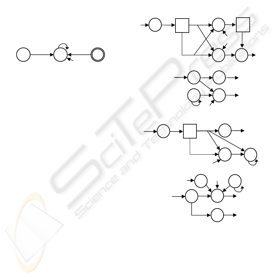
are rational weights. Figure 1
displays a graphical representation of equation (2),
used throughout this paper. When a
ji
(or b
jk
or a
jj
)
takes value 1, it is not displayed in the graph.
Figure 1: Graphical notation for neurons, input channels
and their interconnections.
Using this model, we designed a high-level
programming language, called
NETDEF, to hard-wire
the neural network model in order to perform
symbolic computation. Programs written in
NETDEF
can be converted into neural nets through a compiler
available at www.di.fc.ul.pt/~jpn/netdef/netdef.htm.
NETDEF is an imperative language and its main
concepts are processes and channels. A program can
be described as a collection of processes executing
concurrently, and communicating with each other
through channels or shared memory. The language
has assignment, conditional and loop control
structures (figure Figure
2 presents a recursive and
modular construction of a process), and it supports
several data types, variable and function
declarations, and many other processes. It uses a
modular synchronization mechanism based on
handshaking for process ordering (the
IN/OUT
interface in figure Figure
2). A detailed description
of
NETDEF is found at https://docs.di.fc.ul.pt/ (report
99-5).
The information flow between neurons, due to the
activation function σ is preserved only within [0, 1],
implying that data types must be coded in this
interval. The coding for values of type real within
[-a, a], where ‘a’ is a positive integer, is given by
α(x) = (x + a)/2a, which is a one to one mapping of
[-a, a] into set [0, 1].
Input channels u
i
are the interface between the
system and the environment. They act as typical
NETDEF blocking one-to-one channels. There is also
a FIFO data structure for each u
i
to keep
unprocessed information (this happens whenever the
incoming information rate is higher than the system
processing capacity).
The compiler takes a
NETDEF program and
translates it into a text description defining the
neural network. Given a neural hardware, an
interface would translate the final description into
suitable syntax, so that the neural system may
execute. The use of neural networks to implement
arbitrary complex algorithms can be then handled
through compilers like
NETDEF.
Figure 2: Process construction of: IF b THEN x := x–1.
As illustration of a symbolic module, figure 2
shows the process construction for IF b THEN x := x–
1. Synapse
IN sends value 1 (by some neuron x
IN
)
into x
M1
neuron, starting the computation. Module G
(denoted by a square) computes the value of boolean
variable ‘b’ and sends the 0/1 result through synapse
RES. This module accesses the value ‘b’ and outputs
it through neuron x
G3
. This is achieved because x
G3
bias -1.0 is compensated by value 1 sent by x
G1
,
allowing value ‘b’ to be the activation of x
G3
. This
c
j
a
ji
x
i
x
j
u
k
b
jk
a
jj
OUT
OUT
OUT
-1
2
-1
IN
G
IN
IN
RES
P
x
M1
x
M2
x
M3
x
M4
M
AIN NE
T
-1
OUT
IN
b
RES
x
G1
x
G2
x
G3
M
ODULE G
x
IN
OUT
-1
E
RES
IN
OUT
x
P1
x
P2
x
P3
-1
M
ODULE
P
-
1
-3/2
OUT
IN
x
α
(1)
2
RES
x
E1
x
E2
x
E3
x
E4
M
ODULE
E
IJCCI 2009 - International Joint Conference on Computational Intelligence
398
result is synchronized with an output of 1 through
synapse
OUT. The next two neurons (on the Main
Net) decide between entering module P (if ‘b’ is
true) or stopping the process (if ‘b’ is false). Module
P makes an assignment to the real variable ‘x’ with
the value computed by module E. Before neuron x
receives the activation value of x
P3
, the module uses
the output signal of E to erase its previous value. In
module E the decrement of ‘x’ is computed (using
α(1) for the code of real 1). The 1/2 bias of neuron
x
E2
for subtraction is necessary due to coding α.
The dynamics of neuron x is given by (3).
However, if neuron x is used in other modules, the
compiler will add more synaptic links to its
equation.
x(t+1) = σ( x(t) + x
P3
(t) – x
E3
(t) )
(3)
This resulting neural network is homogenous (all
neurons have the same activation function) and the
system is composed only by linear, i.e., first-order
neurons. The network is also an independent
module, which can be used in some other context.
Regarding time and space complexity, the compiled
nets are proportional to the respective algorithm
complexity.
3 OPERATOR TYPE
PARALLELIZATION
It is possible to insert parallel computation on
certain type expressions. An example follows with
arithmetic expressions. When, say, expression
(a+4)*(b+c) needs evaluation, typical high-level
languages tend to execute it to a sequential fashion.
However, in this case, since each operator will
consist of a neural network, it is possible to execute
all expressions at once and simply wait for the
higher priority expressions to be computed before
executing the lower priority ones. Here we have
three priorities: (i) evaluate the values of the atomic
expressions (‘a’, ‘4’, ‘b’ and ‘c’), (ii) evaluate both
sums (‘a+4’ and ‘b+c’) and finally, (iii) evaluate the
multiplication (see figure 3).
Since there are no operators with side-effects in
NETDEF (nothing like C’s i++) it is safe to fetch the
values of every variable at the same time and
execute these net to compute the final expression
value.
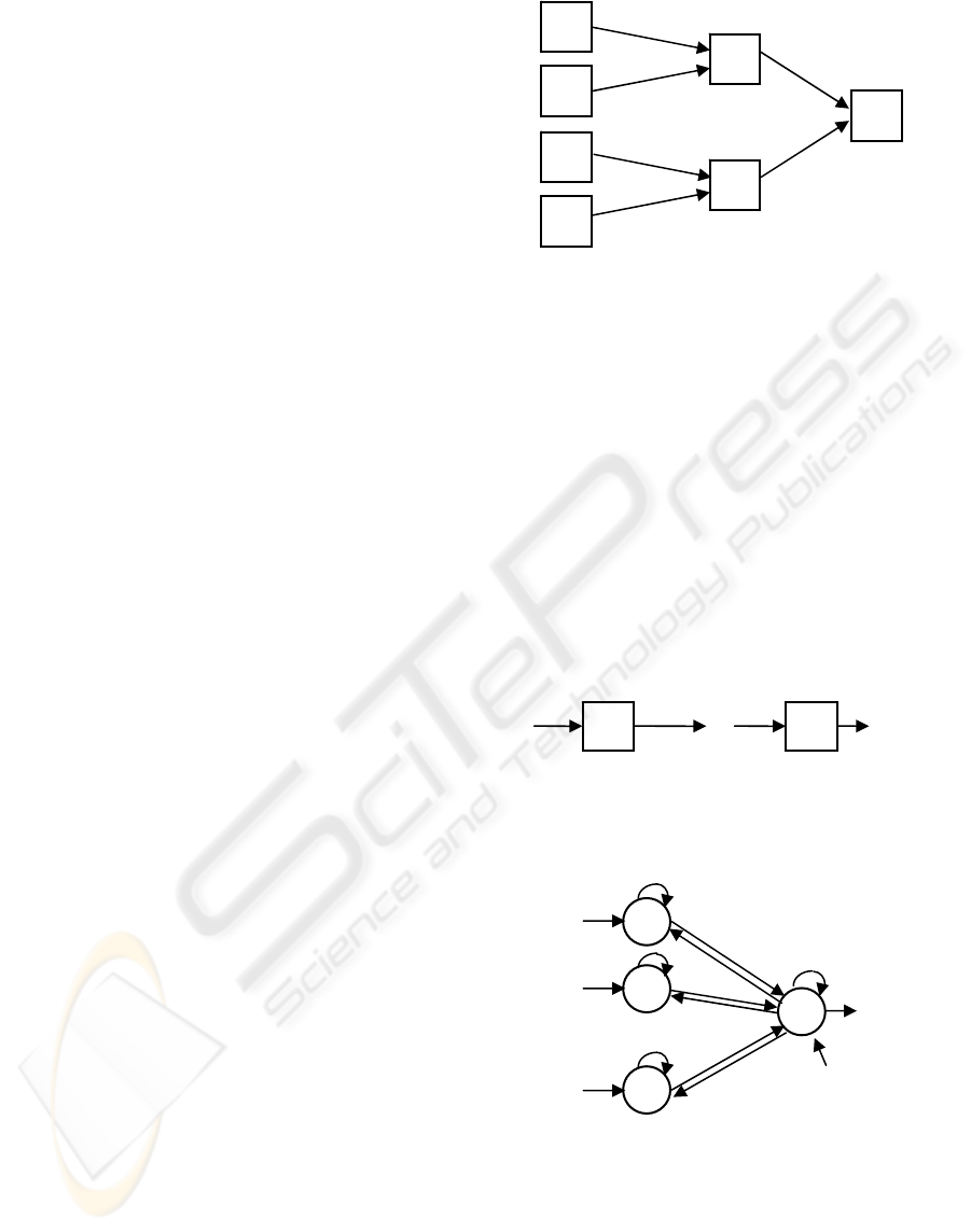
Figure 3: Network scheme for the parallelization of
expression(a+4)*(b+c). To understand its internal
structure check next section’s parallel blocks.
4 PARALLEL BLOCKS
This section deals with controlling the parallel
execution of all neurons to allow sequential
processes.
As seen in figure 2,
NETDEF uses a hand-shaking
mechanism to control each module execution. A
module is connected to their immediate neighbors
via an
IN/OUT signal synchronization. A module only
starts after receiving an IN signal and ends by
outputting an
OUT signal. This allows for a simple
sequential block structure:
Figure 4: A sequential block.
A parallel block can be built based on this next
network:
Figure 5: Synchronizing output signals.
This network waits for the last signal to arrive.
That is, if each of the leftmost arrows indicates the
end of a certain module execution, that signal (again,
a value 1) will be kept within a specific neuron (the
left neurons have a synapse onto themselves with
weight 1). Every signal will be kept on its neuron
until all n neurons have value 1 (due of the –(n-1)
a
4
b
c
+
+
*
OUT
IN
IN
I
1
...
IN
OUT
I
n
-(n-1)
-1
-1
-1
-1
AUTOMATIC PARALLELIZATION IN NEURAL COMPUTERS
399
bias of the right neuron, which is enough to
compensate for n-1 activated neurons). Only when
all n neurons are sending values (meaning that all
previous modules ended their execution), the
negative bias is overcome and the right neuron will
output a 1 while, at the same time, resetting the left
neurons (via the -1 synapses showed above). This
net is useful to synchronize expressions (like those
in the previous section) but also to control
instructions.
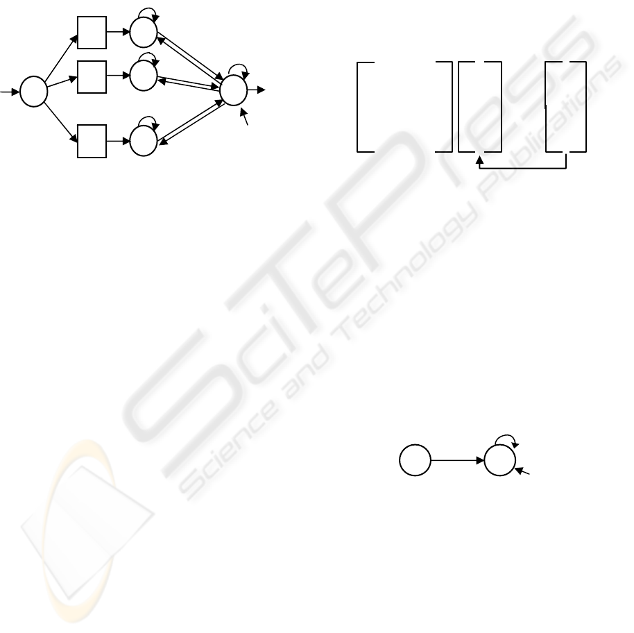
Figure 6: A parallel block.
This parallel block, however, must be explicitly
stated by the programmer, since a sequential or a
parallel block of the same set of instructions denotes,
usually, quite different semantics. The other parallel
features (presented in sections 3 and 5) do not need
any programmer assistance and can be executed
automatically by the compiler and execution
processes.
5 VIRTUAL MACHINE
In section 2, we referred a compiler which translates
high-level algorithmic descriptions into neural nets.
It is straightforward to simulate the execution of
these nets using a regular computer (our own
software can compile and execute the resulting nets).
But, what kind of ‘neural’ hardware would be
adequate to compute these networks? The
NETDEF
language produces modules which communicate via
a small number of channels, but nonetheless the
resulting networks are highly non-planar with
complex topologies. It would not be feasible to
translate this into a 3-D hardware of neurons and
synapses. Besides, every algorithm produces a
different network, so a fixed architecture would be
useful just for a specific problem. It is theoretically
possible to implement a universal algorithm, i.e., to
implement a neural network that codes and executes
any algorithm, but there are easier solutions.
Neural networks can be interpreted as vectors.
Assume a neural network Ψ with n neurons. The
neurons activation at time t can be represented by
vector x
t
= (x
1
(t),x
2
(t)…x
n
(t),1). This vector includes
all the relevant data to define Ψ’s state. The
structure of Ψ is given by a (n+1)×(n+1) matrix M
Ψ
containing all synaptic weights (the extra
row/column is for biases). So, the network dynamics
is given by
x
0
= (x
1
(0),x
2
(0)…x
n
(0),1)
x
t+1
= M
Ψ
. x
t
(4)
which, afterwards, apply function σ to every element
of the resulting vector. Graphically:
Figure 7: Updating the network state.
This implementation is simple and it only uses
sums, products and the σ function. However there
are disadvantages. The typical
NETDEF networks
produce sparse M
Ψ
matrixes resulting on
unnecessary space quadratic complexity.
Our proposed solution is to split the matrix into
smaller tokens of information, namely triples,
looking at a neural network as a list of synapses,
called L
Ψ
.
A classic synapse has three attributes: (a) the
reference to the output neuron (or 1 if it is a bias
synapse), (b) its synaptic value, and (c) the reference
to the input neuron.
Figure 8: This neural network translates to
[(x,a,y), (y,b,y), (1,c,y)].
The list L
Ψ
size is proportional to the number of
synapses. On the worst case (a totally connected
network) it has space quadratic complexity (the
same as the matrix approach). But the usual
NETDEF
network is highly sparse, making it, in practice,
proportional to the number of neurons.
Notice there is no need to keep detailed
information about each neuron; they are implicitly
defined at L
Ψ
. This list, herein, has a fixed size: it is
possible to change the synaptic values dynamically
IN
I
2
I
1
I
n
...
OUT
OUT
OUT
-(n-1)
-1
-1
-1
-1
OUT
x
t+1
=
σ
x
t
M
Ψ
c
a
x
y
b
IJCCI 2009 - International Joint Conference on Computational Intelligence
400

but is not possible to create new neurons or delete
existing ones. There is, however, the possibility of
deactivating a neuron by assigning zero values to its
input and output synapses. With some external
process of neuron activation/deactivation, it would
be straightforward to insert/delete the proper triples
at L
Ψ
. More details can be found in (Neto, 2006)
including how to execute this network
representation.
There are ample possibilities for optimization.
The network modules are not all active at once.
Except for high-parallel algorithms (where the
parallelization was thought and designed by the
programmer and is, therefore, not that important in
this stage) there is only a small number of modules
active at each given moment. So, many triples (those
from the inactive modules) are not used and should
not enter in the next computation step. How can we
easily deduce what triples should be calculated?
Herein, the
IN/OUT synchronization mechanism is
again helpful. Since a certain module M is only
activated after its input neuron receives an activation
signal (i.e., the previous synapse receives a 1) that
means that we should keep the triples of those input
synapses – let’s denote them input triples – as
guards of the set of triples representing the
remaining module structure. So, every time an input
triple is activated, the system will upload the entire
triple structure of that module (notice that this may
or may not include the inner sub-modules,
depending on the number of triples these sub-
modules of arbitrary complexity may represent) and
compute it along with all the other active triples.
When an active module ends its computation, the
output triple (representing the synapse that transfers
the output signal to the input neuron of the next
module) is activated and the system has enough
information to remove the module structure from the
pool of active triples.
Using this mechanism, the number of triples in
execution depends only of the number of active
modules and not in the entire network structure. This
will speed the execution of single modules and
provide a better efficient use of the available parallel
processing power.
6 CONCLUSIONS
Neural networks can be used to compute the
execution of symbolic algorithms. The fact that
neural nets are massive parallel models of
computation, allow us to use this feature in several
ways to speed the calculation of modules and
expressions that do not have precedence over each
other. We have shown two possible uses at this
level: expression parallelization and parallel blocks.
Also, since neural nets can be decomposed into
triplets (each representing a synaptic connection), it
is also possible to speed computation by allocating
sets of synaptic triples into different CPU’s to
calculate the next computing state.
ACKNOWLEDGEMENTS
This work was supported by LabMAg (Laboratório
de Modelação de Agentes) and FCT (Fundação para
a Ciência e Tecnologia).
REFERENCES
Carnell, A., Richardson, D., 2007. Parallel computation in
spiking neural nets, Theoretical Computer Science
[386]1-2, Elsevier, 57–72.
Gruau, F., Ratajszczak, J., Wibe, J., 1995. A neural
compiler, Theoretical Computer Science, 141, 1–52.
Herz, A., Goltisch, T., Machens, C., Jaeger, D., 2006.
Modelling Single-Neuron Dynamics & Computations:
A Balance of Detail and Abstraction, Science, 314,
80–85.
McCulloch, W., Pitts, W., 1943. A logical calculus of the
ideas immanent in nervous activity, Bulletin of
Mathematical Biophysics, 5, 115–133.
Neto, J., Siegelmann, H., and Costa, J., 1998. On the
Implementation of Programming Languages with
Neural Nets, First International Conference on
Computing Anticipatory Systems, 1, 201–208.
Neto, J., Costa, J., and Siegelmann, H., 2003. Symbolic
Processing in Neural Networks, Journal of Brazilian
Computer Society, [8]3, 58–70.
Neto, J. 2006. A Virtual Machine for Neural Computers,
16
th
International Conference of Artificial Neural
Networks, in S. Kollias et al. (eds.), Lecture Notes of
Computer Science 4131, Springer-Verlag, 525–534.
Siegelmann, H. and Sontag, E., 1994. Analog
Computation via Neural Networks”, Theoretical
Computer Science, 131, Elsevier, 331–360.
Siegelmann, H., 1999. Neural Networks and Analog
Computation, Beyond the Turing Limit, Birkhäuser.
AUTOMATIC PARALLELIZATION IN NEURAL COMPUTERS
401
