
Robust Navigation for an Autonomous Helicopter
with Auxiliary Chattering-free Second Order Sliding
Mode Control
S. Vite-Med´ecigo, Ernesto Olgu´ın-D´ıaz and Vicente Parra-Vega
Robotics and Advanced Manufacturing
Research Center for Advanced Studies–CINVESTAV, Saltillo, Mexico
Abstract. This paper presents a novel technic for autonomous flight and naviga-
tion control of AAVs, particularly useful for helicopters. Three servo-loop con-
troller are introduced to yield stable robust regulation. The inner control loop is
based on an LQR regulator designed over the linearized plant at hover to guar-
antee close-loop stability. The middle loop is a feedback linearization controller
based on the close-loop linearized system to cope with the underactuated nature
of the helicopter, by guaranteing an asymptotically stable zero dynamics. Finally
the outer control loop enforces a tracking second-order sliding-mode for cartesian
position and heading navigation outputs. The simplicity of this control proposal
allows easier and intuitive guidelines to tune feedback gains while the chattering-
free sliding-mode fulfills basic robustness properties, ideal for this complex sys-
tems subject to external disturbances like wind gusts.
1 Introduction
Automatic flying vehicles, also known as Autonomous Aerial Vehicle (AAV), repre-
sents a huge field of applicationsin particular for advancedautomatic control techniques
because human intervention is considered difficult or dangerous. There are wide civil
and military interests in helicopters, like traffic surveillance, air pollution monitoring,
area mapping, agricultural applications, exploration, scientific data collection, search
and rescue.
Among the AAVs, the rotary wing AAVs such as the helicopter has the advantage
of having the ability to perform different flight regimes like hover, backward, lateral
of pure vertical flight, in contrast to fix wing such as typical airplanes. However, heli-
copters are underactuated mechanisms whose dynamic model exhibits high nonlinear-
ities with physical parameters hard to measure precisely. The operational versatility of
helicopters requires complex controllers to achieve such flight regimes.
We can classify two type of controllers. One uses the full dynamic modeling with
simple model-free controllers; the second assumes simple dynamic modeling used in
complex controllers design. In the former case, due to the complexity of the full dy-
namic model of helicopters and unknown aerodynamic/aeroelastic parameters, model-
based controllers are hard to implement and then simpler control laws based on lin-
earized plant are preferred. Since this approach is prone to instability due to the un-
Johansson R., Vite-Med
´
ecigo S., Olgu
´
ın-D
´
ıaz E. and Parra-Vega V. (2009).
Robust Navigation for an Autonomous Helicopter with Auxiliary Chattering-free Second Order Sliding Mode Control.
In Proceedings of the 3rd International Workshop on Intelligent Vehicle Controls & Intelligent Transportation Systems, pages 47-56
Copyright
c
SciTePress

knowns of the dynamic plant, an auxiliary ν controller is added, typical PID-like con-
troller, which introduces limited performance because of the well-known limitations of
these PID-like controllers. However this type of studies has been useful to understand
better the complexity and structural properties on real applications because they em-
ploy the full model with simple controllers providing clear intuitive understanding on
the stability properties of the closed-loop system. The latter case uses simpler dynamic
models, based on restrictive academic assumptions, such as the helicopter is constrained
to move only in a subset of ℜ
6
, exhibiting pseudo-flying conditions with model-based
controllers [4]. This approach guarantees very limited performance in real conditions,
with limited scope of real applications.
In this paper, we focus our attention in the full dynamical model of the scalar R/C
X-cell90 helicopter, and propose a novel auxiliary controller based on a chattering-free
sliding modes, which increases the closed-loop performance because it is a tracking-
designed controller with inherent robustness capabilities. This allows to guarantee bet-
ter closed-loop performance in comparison to auxiliary controllers based on PID-like
controllers. Simulations under external disturbances like wind gusts, wherein clearly
verifies the validity of the proposed approach.
2 Relevant Background
Complex helicopter models, [9,12], based in the Newtonian model of a free flying rigid
objet are restricted to measurements on the center of mass, which indeed can vary in
real conditions, neglecting at small velocities the Coriolis effects, thus this model is
not useful in aggressive maneuvers or wide range of operational flight conditions. More
over, dissipative effects on the fuselage are not taken in account that would be important
during the navigation. In [6] this Coriolis effects are taken in account but simplifies the
6-DOF Inertia-Matrix to be completely diagonal. More over, a spring model is included
to describe the main rotor forces mapping to the main body rigid object modeling.
Nonetheless these models neglect the blade’s kinetic energy, which can be up to 20
times the one of the fuselage [1]. Thus, in hover regime this energy must be taken in
account to give rise to a dynamic model of more than the 6 degrees of freedom (DOF)
of a rigid free flying object, showing the complexity of the main rotor itself. This model
is more relevant in practice since it includes this important energy.
On one hand the forces acted in the rigid free flying object (the fuselage) are given
mainly by the forces exerted at the main and tail rotors. The forces at the tail rotor is a
simple thrust in the direction perpendicular to the tail rotor whose magnitude changes
with the tail collective. On the other hand, the main rotor provides 3 Cartesian compo-
nents of the main rotor thrust given by the main rotor collective and two azimuth angles
also known as lateral and longitudinal cyclic. Then, even for the most simplest model,
i.e. 6-DOF, the full system is underactuated because the control dimension is 4.
The problem of control design for this kind of systems even for complex models
including all or some of the full main rotor dynamics as been addressed extensively in
the literature, however the control of the underaction remains open, though it has been
addressed in [2,13]. In particular, [14] proposes LQR-BDU techniques a the linearized
model, concluding a robust regulator in a small neighborhood of the linearized point.
LQR feedback control scheme plus an additional PID-like regulators loop is a pop-
ular choice because the unknown parameters and external disturbances, like gust of
wind, deviates the operational point; however the popular integral-loop may increase
the sensitivity of the system under commonly time-varying disturbances. In this paper,
the additional servoloop is based on a robust chattering-free sliding mode controller to
provide wider operational conditions, with better performance.
3 Mathematical Model
In contrast to the Lagrange method, the equations obtained via Newton’s laws expressed
with velocities and acceleration measured at the body (relative to the body’s frame and
not to the inertial one) result in a simpler representation. The difference in these repre-
sentations arise from the fact that the generalized coordinates needed in the Lagrange
method, while having a physical meaning in the pose, the generalized velocity does
not have a physical meaning and neither the generalized force vector; at least part of
them. Equivalences between these two different representations can be obtained via the
kinematic equation, i.e. using the mapping operator that express the physical meaning
of velocity wrench used in Newton formulation out of the generalized velocity vector
used in Lagrange one [5, 10].
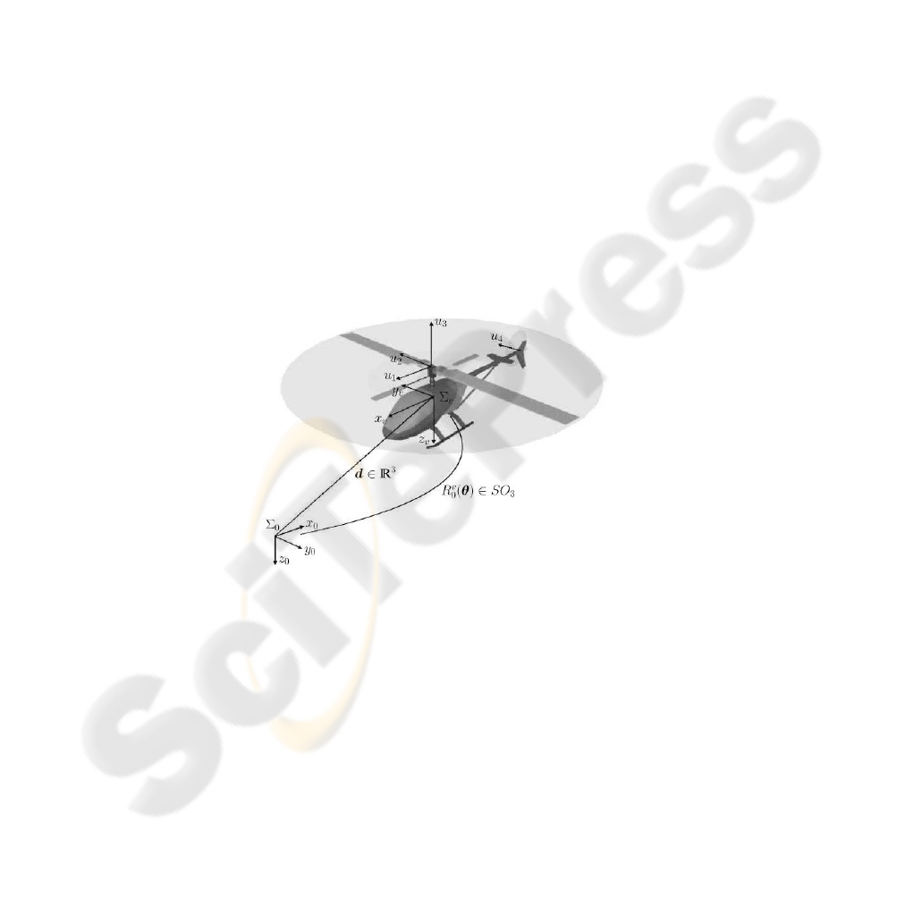
The kinematic of a rigid single body in space is represented only by the pose (posi-
tion and attitude) of the body with respect to an inertial (fixed) frame Σ
0
, where Σ
v
is
the frame rigidly attached to the object. See Fig. 1.
Fig.1. Inercial frame Σ
0
and object frame Σ
v
.
The rotation matrix R
v
0
∈ SO
3
transfers a 3D vector from its representation in
frame Σ
v
to the inertial frame Σ
0
. The generalized position of the object, expressing
both position and attitude of the object is then defined as
q ,
d
θ
v
∈ ℜ
6
(1)
where d = (x, y, z)
T
∈ ℜ
3
is the object inertial position with respect to the
Σ
0
given by the inertial Cartesian coordinates of the origin of frame Σ
v
and θ
v
=
(φ
x
, θ
y
, ψ
z
)
T
∈ [−π, π] × [−π/2, π/2] × [−π, π] is the set of attitude parameters (in
this case the roll-pith-yaw Euler angles) of Σ
v
with respect to Σ
0
. For this very set of
attitude parameter the form of the rotation matrix R has a particular expression that can
be found in either [5, 10]. The vector ν ∈ ℜ
6
is the velocity twist which defines the lin-
ear and angular velocity of Σ
v
expressed in the non-inertial frame Σ
v
, i.e. the velocity
measured from the object
ν ,
v
ω
∈ ℜ
6
(2)
where v = R
v
0
T
˙
d ∈ ℜ
3
is the lineal velocity of the object and ω ∈ ℜ
3
is the angular ve-
locity of frame Σ
v
, both vectors expressed in the non-inertial frame Σ
v
. In strictly math-
ematical sense R
v
0
T
˙
θ
v
6= ω, however there is a relationship given by ω = R
v
0
T
J
θ
˙
θ
v
,
where J
θ
∈ ℜ
3×3
is a linear operator given by attitude parameters. Then a relationship
between ν and ˙q is found as follows
ν = J
v
(q) ˙q (3)
with J
v
(q) ∈ ℜ
6×6
being the linear operator of the kinematic equation. The Kirchhoff
formulation for the equation of motion of a rigid object is nothing but the moment
conservationequations expressed in the non-inertial frame in terms of the kinetic energy
as
d
dt
∂K
∂v
+ ω ×
∂K
∂v
= f (4)
d
dt
∂K
∂ω
+ ω ×
∂K
∂ω
+ v ×
∂K
∂v
= n (5)
where f and n are the forces and torques respectively that acts over the object, including
gravity, dissipative forces and any external input force acting on the object, and K is
the kinetic energy as K =
1
2
ν
T
Mν, where matrix M ∈ ℜ
6×6
is the Inertia Matrix with
respect to the origin of frame Σ
v
, defined as follows:
M ,
mI
3
−m[r
c
×]
m[r
c
×] I
g
(6)
which is by construction constant, positive definite and symmetric M = M
T
> 0. The
terms of this Inertia Matrix are the total mass m of the object, the distance from the
origin of frame Σ
v
to the center of mass of the body r
c
, expressed in the body’s frame,
the inertia moment matrix I
g
computed from the origin of Σ
v
, and the skew symmetric
matrix representation of the cross product [a×]b = a × b.
Equations (4)-(5), after proper algebraic manipulation and using the kinetic energy
expression above, can also be expressed in a single vectorial equation as
M ˙ν + c(ν) = F,
where matrix M ∈ ℜ
6×6
is the Inertia Matrix with respect to the origin of frame Σ
v
,
the vector c(ν) regroups all the nonlinear terms and is known as the Coriolis vector, and

F ,
f
T
, n
T
T
= F
G
+ F
D
+ F
T
is the force wrench consisting in gravity, dissipation
and thrust wrenches respectively.
Because of the quadratic nature in terms of velocity Coriolis vector it can also be
expressed as product of a matrix and the velocity wrench: c(ν) = C(ν)ν. The matrix
C(ν), referred as the Coriolis matrix may have many different representations, but at
last one of them fulfills the skew-symmetry property C(ν) + C(ν)
T
= 0.
F
G
, being the gravity force wrench in the objects frame, can be computed rotating
the gravity influence to the objects frame f
g
= mgR
v
0
T
k. The gravity vector is defined
then as g(q) ,
f
T
g
; 0
T
. Then F
G
= −g(q), where the negative sign comes from the
fact that the positiveness of the vertical axis z
0
is pointing downward, to the center of
the earth, due to convention in vessel engineering.
F
D
are the dissipation aerodynamic forces and these are by nature quadratic and ho-
mogeneous to the velocity wrench. Then a possible approach to model these forces can
be given as F
D
= −D (kνk) ν, where the damping matrix should be definite positive
D > 0 to fulfill passivity [10].
Finally, F
T
are thrust aerodynamical wrench and are given by the influences of the
forces exserted by both rotors. There are 3 forces at the center of the main rotor given
by longitudinal cyclic (u
1
), the lateral cyclic (u
2
) and the collective (u
3
). There is also a
fourth force at the center of the tail rotor (u
4
) (See Figure 1). This mapping is given by
a constant operator B
e
∈ ℜ
6×4
that can be computed from the geometry of the rotors
with respect to vehicle’s frame Σ
v
as F
T
= B
e
u, with u = (u
1
, u
2
, u
3
, u
4
) ∈ ℜ
4
and
B
e
a column full rank matrix.
The dynamic modeling of the helicopter without considering the rotors dynamic is
then given by [10]:
M ˙ν + C (ν) ν + D (k νk) ν + g (q) = B
e
u (7)
ν = J
v
(q) ˙q (8)
which can be expressed is state space form using the state definition x , (q
T
, ν
T
)
T
.
4 Controller Design
A robust control law is necessary due to the environmental nature of AAV, then LQR
approach is preferred because it is an optimal criteria for set-point control while min-
imizing energy consumption [8]. However this technic is based on a linear model or
a linearized one, which means it works as supposed only in the operational point x
o
,
where the linearization was computed with ˜x = x − x
o
:
˙
˜x = A˜x + Bu (9)
y = C ˜x (10)
In the case of the system (7)-(8) the state realization yields to
A(x) =
"
∂
∂q
J
−1
v
(q)ν
J
−1
v
(q)
−M
−1
∂
∂q
g(q)
−M
−1
[C(ν) + D (kνk)]
#
∈ ℜ
12×12
(11)

B =
0
M
−1
B
e
∈ ℜ
12×4
, C =
I 0
∈ ℜ
6×12
(12)
Remark 1. Clearly, (12) indicates that CB = [0] ∈ ℜ
6×4
.
For the particular case where the operation point is hover, i.e. x
o
=
q
T
d
; 0
and q
d
=
(x
d
, y
d
, z
d
, 0 , 0, 0)
T
the state matrix becomes constant:
A =
"
0 I
−M
−1
h
∂
∂q
g(q)
i
0
#
∈ ℜ
12x12
(13)
for the same pair (B, C). From (13) it can be seen that the linearized model at hover
operationalpoint has all the eigenvaluesat the origin. This is due to the double integrator
nature of the system and the fact that the aerodynamic dissipation forces are quadratic
to the velocity which becomes null at the steady state. This explains the high degree of
instability of such systems.
Remark 2. Notice that the pair (A, B) is controllable, then a linear state feedback (u =
−Kx) would enforce a desired closed-loop system stability and performance at the
operation state x
o
[3].
Remark 3. The product CAB = M
−1
B
e
∈ ℜ
6×4
is column full rank constant matrix,
and column full rank matrix elsewhere: CA(x)B = J
−1
v
(x
1
)M
−1
B
e
∈ ℜ
6×4
.
4.1 Feedback Linearization
Stability of the equilibrium point x
o
is only local and valid only in its very narrow
neighborhood. When the dynamic model deviates or the system is subject to bounded
unmodeled dynamics or bounded disturbances. To cope with that an auxiliary feedback
control is commonly proposed [2],
u = −Kx + v (14)
where K is computed via LQR feedback scheme and v is an additional auxiliary control
input. Then, the linearized close-loop system can be written as
˙x = [A − BK] x + Bv (15)
¯y =
¯
Cx (16)
where ¯y is only a part of the originally output (y = q), defined, as the Cartesian position
and heading only, excluding the roll and pitch attitude angles: ¯y , (x, y, z, ψ
z
)
T
. The
output matrix
¯
C = [C
1
0] ∈ ℜ
4×12
with C
1
∈ ℜ
4×6
has raw full rank. Notice that
¯
CB = [0] ∈ ℜ
4×4
still holds, consequently the first and second time derivatives of the
new output become
˙
¯y =
¯
CAx (17)
¨
¯y =
¯
CA [A − BK] x +
¯
CABv (18)

Remark 4. Matrix
¯
CAB = C
1
M
−1
B
e
∈ ℜ
4×4
is full-rank invertible matrix, thus
stable zero dynamics arise, that is the roll and pitch attitude angles are stable, [7].
The Feedback Linearization controller (FL), issued from eq. (18) would have the
form
v =
¯
CAB
−1
¯v −
¯
CA [A − BK] x
, (19)
yielding to a closed-loop system
¨
¯y = ¯v, as reported in [2]. However this is rather
awkward since the LQR state feedback (−Kx) is canceled in (14) by this second loop.
Since it is preferable to maintain an optimal stabilizable regulator such as the LQR in
the control loop a Partial Feedback Linearization (PFL) is proposed as:
v =
¯
CAB
−1
¯v −
¯
CA
2
x
(20)
which delivers a second order coupled linearized close-loop system
¨
¯y = ¯v −
¯
CABKx (21)
Notice that dynamics −
¯
CABKx represents the a residual coupled dynamics introduced
by the optimal LQR regulator and because of the underactuated nature of this system.
4.2 Sliding-Mode Control
Let ∆¯y = ¯y
d
− ¯y be the output tracking error, where y
d
is the desired output signal, and
choosing the new second order sliding-mode control law ¯v given by
¯v ,
¨
¯y
d
− α∆
˙
¯y + βs
0
e
−βt
− K
i
tanh(σs
q
) − K
d
s
r
(22)
for large enough gains K
d
, K
i
and small error on initial conditions, with s
r
= s
q
+
K
i
R
sgn(s
q
), s
q
= s − s
d
, s = ∆
˙
¯y + α∆¯y and s
d
= s
0
e
−βt
, s
0
= s(t
0
). The
function tanh(∗) stands for a the sigmoid hyperbolic tangent function with σ > 0, not
necessarily large. Then, the complete control law is given by
u =
¯
CAB
−1
¨
¯y
d
− α∆
˙
¯y + βs
0
e
−βt
− K
i
tanh(σs
q
) − K
d
s
r
−
¯
CA
2
x
− Kx
(23)
Substituting (23) into (9) yields
˙s
r
= −K
d
s
r
−
¯
CABKx − K
i
Z (24)
for bounded Z = tanh(σs
q
) − sgn(s
q
). Finally, we can state the main result.
Theorem 1. Consider (23) into (9), then the closed loop (24) gives rise to robust ex-
ponentially stable dynamics of tracking errors, under a chattering-free second order
sliding modes for all time, with stable zero dynamics.
Proof. It follows closely [11], QED.
Remark 5. The state feedback stabilize locally the operation point, decouples the close-
loop dynamics of the lateral, longitudinal, vertical, and heading navigation and pre-
serves stability of the zero dynamics. Additionally, the auxiliary control input enables a
wider operational region by adding robustness to the overall closed loop control.
5 Results
Consider the nonlinear model of an X-cell90 R/C helicopter. The linear model is com-
puted, for simulation simplification, at the operating point x
o
= (0, 0, 0, 0, 0, 0)
T
. In
Table 1 initial conditions and gain tuning for the output feedback sliding mode are
shown. For comparison purposed, simulation using Matlab are also performed com-
muting the auxiliary control (14) for a properly tuned PD control.
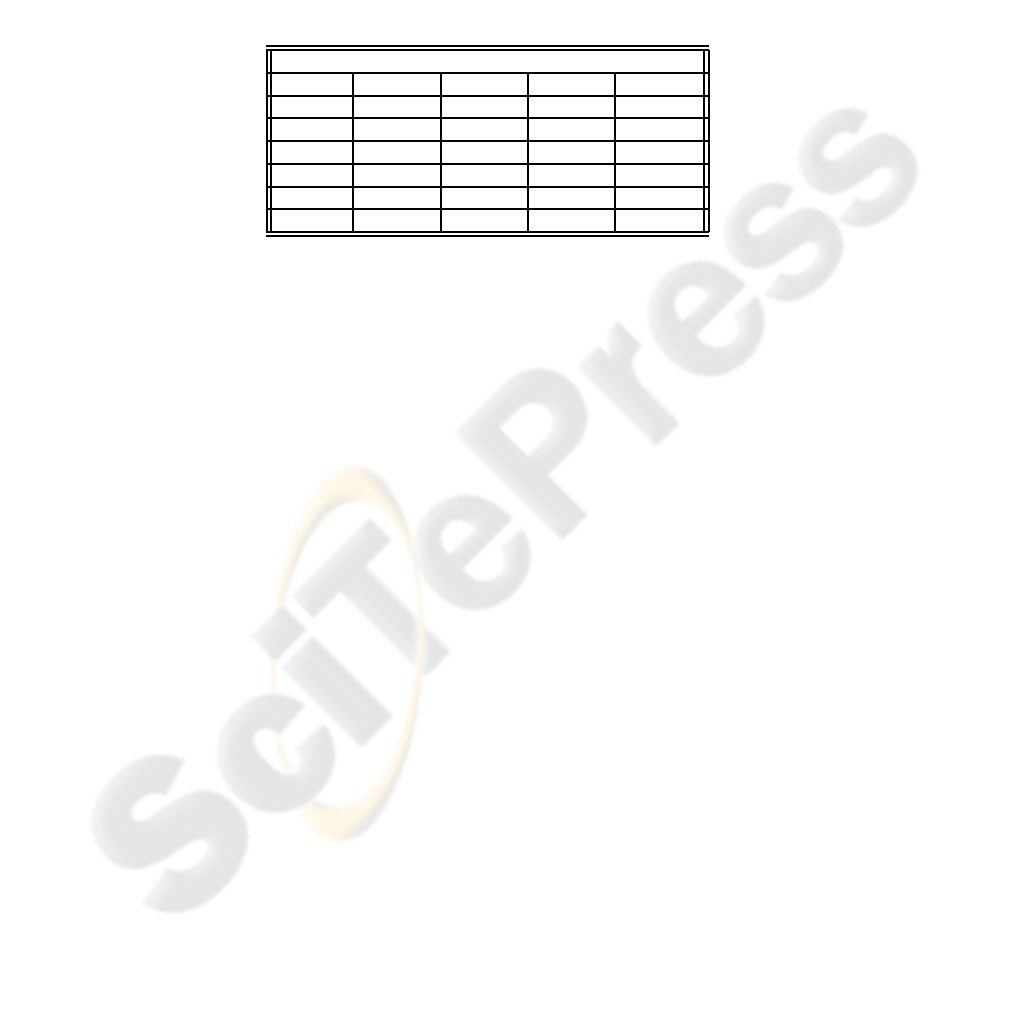
Table 1. Initial conditions and tuning gains for the sliding-mode control.
Initial conditions & SMC-Gains
x y z ψ
q
0
-2.1 1.05 0.11 0
˙q
0
0 0 0 0
α 3.15 3.15 4.5 15
β 1 1 1 1
k
d
15.6 15.6 56.16 234
k
i
3.51 3.51 27.8 52.65
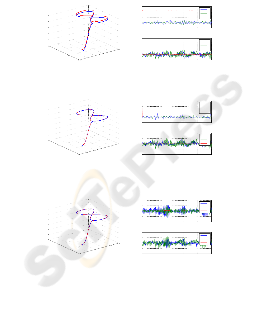
Figure 2 shows the 3D trajectory and the tracking error of both position and attitude
for the helicopter when the control law is the two servo-loop, similar to the one pre-
sented in [2] (FL-PD), consisting in a Feedback Linearization (which also cancels de
LQR inner loop) and a PD controller. As it can be seen this PD controller cannot reject
constant disturbances as gravity. Figure 3 shows the same trajectory tracking with the
proposed Sliding-Mode robust controller in the place of the PD above (FL-SM). This
controller consist in a Feedback Linearization and a second order Sliding-Mode output
feedback. It can be seen a good performance on the desired position tracking, including
the heading (yaw angle), even in the presence of random disturbance forces (for gust of
winds). The roll and pitch angles, which define the zero dynamics, are stable, which is
in accordance with the feedback linearization design. Figure 4 shows also the trajectory
tracking as in the previous Figures. The difference here is that in this case the middle
loop does not cancel the LQR inner loop, and the residual dynamics are coped by the
outer second order Sliding-Mode loop. This controller, given by (23), is called in this
work as LQR-PFL-SM. Evident differences in the performance of the FL-PD and the
FL-SM can be seen mainly because the PD cannot overcome constant disturbances as
the gravity effect. Small differences between the FL-SM scheme and LQR-PFL-SM
one can be seen at the magnitude level of the Cartesian position tracking error where
are smaller in the second, because the Sliding mode acts since the initial conditions,
tracking almost perfectly the desired trajectory. In attitude there are no significative
differences founded.
6 Conclusions
Control of autonomous helicopters in the presence of environmental and system un-
certainties is a challenging task. These uncertainties not only modify the dynamics be-
−4
−2
0
2
4
6
0
2
4
6
−0.5
0
0.5
1
1.5
2
3D Position
0 20 40 60 80 100
−0.05
0
0.05
0.1
0.15
Position error (q
1
, q
2
, q
3
)
e
1−3
[m]
e
1
e
2
e
3
0 20 40 60 80 100
−0.1
0
0.1
0.2
0.3
Attitude error (q
4
, q
5
, q
6
)
t [s]
e
4−6
[rad]
e
4
e
5
e
6
Fig.2. Space position trajectory tracking in 3D and pose tracking errors for a FL-PD control law.
−4
−2
0
2
4
6
0
2
4
6
−0.5
0
0.5
1
1.5
2
2.5
3D Position
0 20 40 60 80 100
−0.02
0
0.02
0.04
0.06
Position error (q
1
, q
2
, q
3
)
e
1−3
[m]
e
1
e
2
e
3
0 20 40 60 80 100
−0.2
−0.1
0
0.1
0.2
Attitude error (q
4
, q
5
, q
6
)
t [s]
e
4−6
[rad]
e
4
e
5
e
6
Fig.3. Space position trajectory tracking in 3D and pose tracking errors for the FL-SM control
law.
−4
−2
0
2
4
6
0
2
4
6
−0.5
0
0.5
1
1.5
2
2.5
x [m]
3D Position
y [m]
z [m]
0 20 40 60 80 100
−1
−0.5
0
0.5
1
x 10
−3
Position error (q
1
, q
2
, q
3
)
e
1−3
[m]
e
1
e
2
e
3
0 20 40 60 80 100
−0.2
−0.1
0
0.1
0.2
Attitude error (q
4
, q
5
, q
6
)
t [s]
e
4−6
[rad]
e
4
e
5
e
6
Fig.4. Space position trajectory tracking in 3D and pose tracking errors for LQR-PFL-SM control
law.

havior of the system, but also the trim inputs themselves. What is therefore needed
is a viable controller capable of simultaneously accommodating all coupling features,
parametric uncertainties, and trim errors. State representation is necessary to perform
both tangent linearization for the design of an ideal Optimal stable State Feedback and
Partial Feedback Linearization for output decoupling and underaction restrictions. The
underactuated nature and the use of some part of the Feedback Linearization control in-
duce undesirable residual dynamics. A second order model-free Sliding-Mode is used
to guarantee robust regulation, while preserving zero dynamic stability. Representative
simulations provide appreciation of the validity of the proposed approach.
References
1. Avila Vilchis, J.C.: Mod´elisation et Commande d’H´elicopt`ere, PhD dissertation, Labora-
toire d’Automatique de Grenoble (LAG), Septembre 2001, Institut National Polytechnique
de Grenoble (INPG), France
2. Bergerman, Marcel; Amidi, Omead; Miller, James Ryan; Vallidis, Nicholas & Dudek, Todd:
Cascaded Position and Heading Control of a Robotic Helicopter, Proceedings of the
2007 IEEE/RSJ International Conference on Intelligent Robots and Systems, San Diego,
CA, USA, Oct 29 - Nov 2, 2007.
3. Chen, Chi-Tsong: Linear System Theory and Design, Third Edition, 1999, ISBN:0-19-
511777-8.
4. Dzul, A.; Lozano, R. & Castillo: Adaptative Altitude Control for a Small Helicopter in
Vertical Flying Stand, Proc. of IEEE Conference on Decision and Control, Maui, Dec. 2003.
5. Fossen, Thor Inge: Guidance and Control of Ocean Vehicles, Chichester, John Wiley and
Sons Ltd, University of Trondheim, Norway, 1994.
6. Gavrilets, V.; Mettler, B. & Feron, E.: Nonlinear model for a small-size acrobatic helicopter,
in Proceedings of AIAA Guidance Navigation and Control Conference, Montreal, Quebec,
Canada, August 2001.
7. Isidori, Alberto: Nonlinear Control Systems, Springer-Verlag, London 2003, 3nd ed. ISBN:
3540199160
8. Lin, Feng: Optimal Control Design: An Optimal Control Approach, John Wiley & Sons,
Ltd, 2007, ISBN:978-0-470-03191-9.
9. Mahony, R.; Hamel, T. & Dzul, A.: Hover Control via Lyapunov Control for an Autonomous
Model Helicopter, Proc. of IEEE Conference on Decision and Control, Phoenix, Dec. 1999.
10. Olgu´ın-D´ıaz, Ernesto; Rubio, Luis; Mendoza, Alejandro; G´omez, Nestor & Benes, Bedrich:
Animacin Virtual en 3D de un helicptero de R/C a escala, 3ra Conferencia Iberoamericana
en Sistemas, Ciberntica e Informtica (CISCI 2004). Orlando, FL, July 2004.
11. V. Parra-Vega, S. Arimoto, Y.H. Liu, G. Hirzinger, and P. Akella: Dynamic sliding PID con-
trol for tracking of robot manipulators: Theory and experiments, IEEE Transaction on
Robotics and Automation, Vol. 19, No. 6, pages 976 985. December 2003.
12. Shim, D.H.; Koo, T.J.; Hoffmann, F. & Sastry, S.: Comprehensive Study of Control Design
for an Autonomous Helicopter, Proc. of IEEE Conference on Decision and Control, Tampa.
1998.
13. Spong, M. W.: Underactuated Mechanical Systems, in Control Problems in Robotics and
Automation, B. Siciliano and K. P. Valavanis Eds., LNCIS, vol. 230, pp. 135–150, Springer
Verlag, London, 1998. http://citeseer.ist.psu.edu/spong98underactuated.html
14. Vite-Med´ecigo, S. & Olgu´ın-D´ıaz, Ernesto: Robust Tracking and Disturbances Rejection
with Robust LQR via BDU for a R/C Helicopter, CIIIEE 2008 - ITA, November 2008,
ISBN:978-607-95060-1-8
