PATH PLANNING WITH MARKOVIAN PROCESSES

Istvan Szoke, Gheorghe Lazea, Levente Tamas, Mircea Popa and Andras Majdik

Technical University of Cluj-Napoca, Daicoviciu Street, Cluj-Napoca, Romania

Keywords: Path planning, Navigation algorithms, Mapping, Mobile robots, Markovian processes.

Abstract: This paper describes the path planning for the mobile robots, based on the Markov Decision Problems. The

presented algorithms are developed for resolving problems with partially observable states. The algorithm is

applied in an office environment and tested with a skid-steered robot. The created map combines two

mapping theory, the topological respectively the metric method. The main goal of the robot is to reach from

the home point to the door of the indoor environment using algorithms which are based on Markovian

decisions.

1 INTRODUCTION

The first step in mobile robot navigation is to create

or to use a map and to localize itself in it (Thrun,

2003). An autonomous agent has to have the

following abilities: map learning or map creating,

localization and path planning. The map

representation can be metric or topological

(Borenstein, 1996). In the case of the metric

representation, the objects are replaced with precise

coordinates, the disadvantage of this representation

is that the precise distances can be very hard

calculated, the map inaccuracies and the dead-

reckoning errors are appearing often. The

topological representation only considers places and

the relations between them, its disadvantages would

be the unreliable sensors which can not detect

landmarks and perceptual aliasing. The second step

in an agent’s navigation process is the localization,

which is strongly dependent to the map learning

phase. This problem is common known as,

Simultaneous localization and mapping (SLAM).

SLAM is of one of the most important researched

subfields of robotics (Fox, 2003). To plan a route to

a goal location, the agent must be able to estimate its

position. The most well known methods to do this,

are the relative and absolute position measurements

(Thrun, 2004). For the relative position

measurements the most used methods are the

odometry and inertial navigation, respectively for

the absolute position estimation, the active beacons,

artificial and natural landmark recognition and map-

based positioning (Thrun, 2003). Path planning is

defined as follows: is the art of deciding which route

to take, based on and expressed in terms of the

current internal representation of the terrain.

The definition of the path finding: the execution

of this theoretical route, by translating the plan from

the internal representation in terms of physical

movement in the environment.

2 PATH PLANNING PROCESS

The effectiveness of a search can be measured in

three ways. Does it bring a solution at all, it is a

good solution (the one with a low path cost), and

what is the search cost associated with the time and

memory required to find a solution. The total cost of

a search is defined as the sum of the path cost and

the search cost. Route finding algorithms are used in

a variety of applications, such as airline travel

planning or routing in computer networks. In the

case of the robot navigation, the agent can move in a

continuous space with an infinite set of possible

actions and states. In case of a circular robot which

is moving on a flat surface, the space is two-

dimensional, but in case of a robot that has arms and

legs, the search space will be many-dimensional.

2.1 Markovian Processes

These kinds of processes integrate topological and

metric representation as well, utilizing both action

and sensor data in determining the robot position

(Cassandra, 1996). Bayes rule is used to update the

479

Szoke I., Lazea G., Tamas L., Popa M. and Majdik A.

PATH PLANNING WITH MARKOVIAN PROCESSES.

DOI: 10.5220/0002209704790482

In Proceedings of the 6th International Conference on Informatics in Control, Automation and Robotics (ICINCO 2009), page

ISBN: 978-989-674-000-9

position distribution after each action and sensor

reading (Koenig, 1996). In a Markov model actions

occur in discrete time. To solve a Markov Decision

Problem requires calculating an optimal policy in a

stochastic environment with a transition model

which satisfies the Markovian property.

2.2 Markov Decision Problem

The problem of calculating an optimal policy in a

stochastic environment with a known transition

model is called a Markov decision problem

(MDP). It can be expressed, that a problem which

has the Markov property, its transition model from

any given state depend only on the state and not on

previous history. Knowledge of the current state is

all that is required in making a decision. A transition

model is one which gives, for each state s and action

a the resulting distribution of states if the action a

was executed in s. A Markov decision process is a

mathematical model of a discrete-time sequential

decision problem (Littman, 2009). MDP is defined

as a four tuple

〉〈 RPAS ,,,

(Regan, 2005), where

is the finite set of environment states,

A is the set of

actions,

is the set of action dependent transition

probabilities,

is the reward function.

RASR →×:

is the expected reward for taking

each action in each state. To maximize the expected

reward over a sequence of decisions is the main goal

of this problem. In an ideal case, the agent should

take actions that maximize future rewards. In an

MDP, the expected future reward is dependent only

on the current state and action, so it must exist a

stationary policy which will guarantee that the

maximum expected rewards are received, if taken

starting from the current state. The goal of any

method to solve a MDP is to identify the optimal

policy. The optimal policy is one that will maximize

the expected reward starting from any state. If we

would enumerate all of the possible policies for a

state space, and then pick the one with the maximum

expected value function, the method would be

intractable, because the number of policies is

exponential in the size of the state space. The

traditional approach to solving sequential decision

problems is dynamic programming. For applying

this type of programming we need precise

information about

, the transition probabilities and

, the reward function. Unfortunately, dynamic

programming is computationally expensive in large

state spaces.

2.2.1 Value Iteration Algorithm

This algorithm is used to calculate the optimal

policy for the given environment. The main idea of

the algorithm is to calculate the utility for each of

the states, note with U(state). These utility values

are used for select an optimal action in each state.

∑

⋅+←

)(max)()(

jUMiRiU

(1)

Where R is called the reward function,

the transition model, the probability of reaching state

j if action a is taken in state i, and U is the utility

estimate. It’s an iterative algorithm, as

∞

>−t

, the

utility values will converge to stable values.

Equation (1) is the basis for dynamic programming,

which was developed by Richard Bellman (Russell,

1995). Using this type of programming sequential

decision problems can be solved.

function VALUE_ITERATION (MDP)

input: MDP with states S,

transition model T,

reward function R

repeat

U = U’

for each state s do

∑

⋅+←

)(max)()(

jUMiRiU

until close enough(U,U’)

return U.

2.2.2 Policy Iteration Algorithm

After the utility values are calculated for all the

states, the corresponding policy is calculated using

the equation (2).

∑

⋅=

jUMipolicy )(maxarg)(

(2)

The basic idea of the algorithm is that by picking

a policy, then calculate the utility of each state given

that policy. The policy is updated after the new

utility is inserted in the equation (3). The RMS

(Root Mean Square) (Russell, 1995) method is used,

to know how many iterations has to be done. The

RMS error of the utility values are compared to the

correct values.

function POLICY_ITERATION (MDP)

input: MDP with states S,

transition model T,

reward function R

ICINCO 2009 - 6th International Conference on Informatics in Control, Automation and Robotics

480

repeat

U = Policy_Evaluation(

,U,MDP)

unchanged?=true

for each state s do

∑

⋅=

jUMipolicy )(maxarg)(

unchanged?=false

until unchanged?

return

2.3 Partially Observable Markov

Decision Problem (POMDP)

This problem like the simple MDP is part of the

sequential decision problems family. This can occur

if the agent’s environment is an inaccessible one,

which means that, there is not enough information in

order to determine the state or the associated

transition probabilities, which means that the agent

cannot directly observe that state. As a solution to

this problem a new MDP has to be constructed,

where the probability distribution plays the role of

the state variable. It will end in a new state space,

which will have real value probabilities, but they are

infinite. For real-time applications even MDPs are

hard to compute, and POMDP need approximations

in order to obtain the optimal policy. Due to the fact

that the agent doesn’t have direct access to the

current state, the POMDP algorithms need the whole

history of the process, which means that it will lose

it’s Markovian property. This step is replaced by

maintaining a probability distribution over all of the

states, it gives us the same result as if we would

keep the entire history. Between decisions the state

can change, unlike in an MDP where state changes

occur just due decisions. A variety of algorithms

have been developed for solving POMDP. The

Whitness algorithm (Littman, 1994) finds the

solution using value iteration, it has been used with

16 states. In case of a more complex state space this

algorithm would not be efficient. Another approach

by (Littman, 1995), is a hybrid one, which is able to

determine high quality policies with approximately

100 states. The realistic problems usually require

thousands of states, so questions to this field remain

open (Regan, 2005).

3 EXPERIMENTAL RESULTS

The described algorithm in this paper was tested

using MobileSim simulator. The Pioneer AT robot’s

starting point is the Home Point situated in the first

cell of the map. The robot has to reach the goal point

which is the door of the room. The first step was to

create the map of the room, where to robot will

navigate. The size of the room is 7m wide and 8.5m

long. The area of the room was divided in cells with

area of

. In Figure 1, the created map can be

seen, with the most representative points, like the

Home Point and the Goal Point. The other visible

objects from the map, are obstacles like desks,

shelves and supportive walls.

Figure 1: The map of the office environment.

The cells which represent an obstacle, their

utility is zero, for the other cells, the iterative

algorithm computes until the value between two

consecutive utility value, for the same cell, is not

more than 0.015. The initial value for a cell is -0.04,

the utility value for the Goal Point is 1, and for a

state which should be avoided, it has a value of -1.

In a real world environment a state with utility -1,

can be a whole in the ground or a state, from where

the robot would get easily lost and use all of its

power, due to this fact the agent must be able to

reach his goal. The path shown in Figure 2, is the

most shortest, what the robot can have. In order to

avoid to get close to the state which has a utility of -

1, the presented algorithm was applied to obtain

another path. The scope of the path which will be

obtained is to not have immediate neighbours to the

cell which has utility of -1.

Figure 2: The shortest path.

PATH PLANNING WITH MARKOVIAN PROCESSES

481

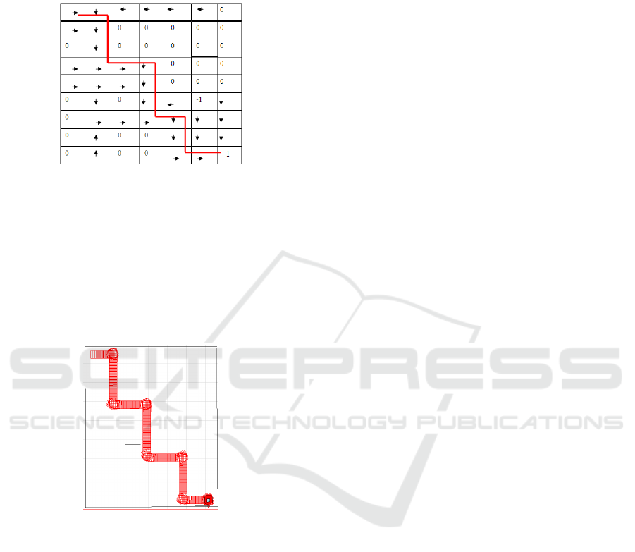
After 20 iterations of the Value Iterative

algorithm, the final utility values were obtained. In

Figure 3, the policies are represented, which were

obtained after applying the Policy Algorithm.

Figure 3: The optimal policy values.

The cells with a higher utility value are more

valuable for this algorithm than the states with a

lower utility value. As shown in Figure 3, the

optimal path has been found, the robot achieving to

the door without getting close to the cell with utility

-1, state which gets the lowest global reward.

In Figure 4, is represented the found path after

testing with MobileSim.

Figure 4: The found path using the presented algorithms.

The agent obtained an autonomous behaviour as

presented in Figure 4 successfully avoids obstacles

and the state with utility -1, it reach to the goal point

which is the door of the office environment. As

shown in Figure 2, the shortest path is not the path

with the least cost (LaValle, 2006).

4 CONCLUSIONS

The main focus of this paper was to present the

algorithms which are solving MDPs for path

planning in mobile robots navigation. In a well

known environment and with all the states

observable, the agent is able to avoid obstacles and

to navigate to the desired point.

5 FUTURE WORK

It is intended to create the map of the environment in

a dynamic way. By the advance of the robot, the

map would be created using the fusion of the data

obtained by multiple sensors. The map will contain

dynamic objects as well, human beings, which will

have to be recognized and inserted in the map and to

determine the projected positions for them.

REFERENCES

Cassandra, T., Kaelbing L., Kurien, J., 1996. Acting under

uncertainty: Discrete bayesian models for mobile-

robot navigation. IEEE/RSJ International Conference

on Intelligent Robots and Systems.

Fox, D., Hightower J., 2003. Bayesian Filtering for

Location Estimation. IEEE Pervasive Computing, vol.

2, no. 3, pp. 24-33, doi:10.1109/MPRV.2003.1228524.

LaValle, S., 2006. Planning algorithms. Cambridge

University Press.

Littman, M,. 1994. The Whitness algorithm: Solving

partially observable Markov decision processes. Tech.

Rep. CS-94-04

Littman, M. L., 2009. A tutorial on partially observable

Markov decision processes. Journal of Mathematical

Psychology.

Regan, K., 2005. The advisor-POMDP: A principled

Approach to Ttrust through Reputation in Electronic

Markets. Proceedings of the third annual conference

on privacy, security and trust, PST..

Thrun, S., 2003. Learning Occupancy Grid Maps with

Forward Sensor Models. Autonomous Robots, v.15

n.2, p.111-127.

Thrun, S., Burgard, W., 2004. A Probabilistic Approach to

Concurrent Mapping and Localization for Mobile

Robots. Springer Netherlands.

ICINCO 2009 - 6th International Conference on Informatics in Control, Automation and Robotics

482