IMAGE UNDERSTANDING USING SELF-SIMILAR SIFT FEATURES
Nils Hering, Frank Schmitt and Lutz Priese
Institut for Computervisualistics, University of Koblenz, Universit¨atsstrasse 1, Koblenz, Germany
Keywords:
SIFT features, Self-similar.
Abstract:
In this paper we present a new method to group self-similar SIFT features in images. The aim is to automat-
ically build groups of all SIFT features with the same semantics in an image. To achieve this a new distance
between SIFT feature vectors taking into account their orientation and scale is introduced. The methods are
presented in the context of recognition of buildings. A first evaluation shows promising results.
1 INTRODUCTION
This work emerged out of the PosE-Project of the
University of Koblenz
1
. The aim of PosE is the de-
velopment of fast algorithms for determination of the
pose (position and orientation) of a camera in a known
3d-modelled scene. For this, prominent features are
annotated in a 3d-model of the scene and matched
against the camera images. A feature is called promi-
nent if it can be easily computed from the image and
is significant in the 3d-model. One possibility for
prominent features are groups of self-similar SIFT
features.
SIFT (Scale Invariant Feature Transform) is an al-
gorithm for extraction of “interesting” image points,
the so called SIFT features. SIFT is commonly used
for matching objects between spatially (e.g. in stereo
vision) or temporally displaced images. In this paper
we instead use SIFT for finding groups of self sim-
ilar features in one image. We will show that there
is a connection between feature representation of ob-
jects on SIFT data level and their semantics in the im-
age. SIFT data inside, e.g., a natural tree should form
a well-defined group of self-similar SIFT features as
well as the SIFT data of, e.g., window sills or cross-
bars. Those groups with a different semantics shall be
distinguishable and some hints on the semantics shall
be possible on the data level. To achieve this a simple
grouping by the distance in Euclidean space is insuf-
ficient and a new topology will be introduced.
1
This work was supported by the DFG under grant
PR161/12-1 and PA 599/7-1
SIFT, SIFT features, and variations of SIFT are
used in several scientific papers. First of all there is
the work of David Lowe who developed SIFT (Lowe,
1999), (Lowe, 2003).
Slot and Kim (Slot and Kim, 2006) use SIFT fea-
tures for object class detection by clustering of similar
features. They use spatial locations, orientations and
scales as similarity criteria to cluster the features. The
regions in which the clustering takes place (the spa-
tial locations) are selected manually. In those regions
clusters are build by a grouping via a “low variance”
criteria in “scale-orientation space”. The main differ-
ence to our approach is their usage of spatial loca-
tions and our usage of distance measures concerning
the feature vectors.
There are other works in which variations of SIFT
or alternatives are presented. The PCA-SIFT of
Ke and Sukthankar (Ke and Sukthankar, 2004) is a
method which uses “Principal Components Analy-
sis” to get keypoint descriptors more easily. Bay,
Tuytelaars and Van Gool developed SURF (Bay et al.,
2006), where features can be computed and compared
much faster than in other approaches.
SIFT features or other parts of SIFT are used in
other contexts, too. Goshen and Shimshoni (Goshen
and Shimshoni, 2006) use SIFT features for the effi-
cent estimation of a matrix. Chum and Matas (Chum
and Matas, 2005) employe the distance ratio of SIFT
features as an example for a measure to advance the
assignment in the RANSAC algorithm (Fischler and
Bolles, 1987).
114
Hering N., Schmitt F. and Priese L. (2009).
IMAGE UNDERSTANDING USING SELF-SIMILAR SIFT FEATURES.
In Proceedings of the Fourth International Conference on Computer Vision Theory and Applications, pages 114-119
DOI: 10.5220/0001753501140119
Copyright
c
 SciTePress

2 SIFT
In this section we give a short overview of the SIFT
algorithm. SIFT extracts characteristic features out of
a greyscale image. These features are described by
a 128-dimensional vector, an orientation, and a scale.
Using the Euclidean distance between SIFT vectors a
feature can be recognized in different images invari-
ant to scale and rotation.
SIFT first scales the input image in a set of differ-
ent resolutions. For each resolution a set of gaussian
smoothings with different variance values is com-
puted. Each of these sets is called an octave. After-
wards a set of difference images is computed for each
set of gaussians by subtracting the neighbour images
in the smoothing sets resulting in a set of Difference
of Gaussian (DOG).
In the next step a minima and maxima search in
the difference images is applied by comparing each
pixel with its eight neighbours in the image and the
nine neighbours in each neighbour image (Fig.1).
Scale
Figure 1: Comparing the neighbour pixels.
From these minima and maxima the keypoints are
chosen. Then for each chosen keypoint a SIFT feature
is generated consisting of four attributes:
• The x- and y-coordinate in the image.
• The level of scale.
• The main orientation of the feature.
• A 128 dimensional description vector.
The range of the level of scale depends on the size
of the image. In our examples of images with a size of
1024x768 it ranges between zero and about 100. The
maximum is reached e.g. at features in the center of a
square with a side length of nearly 768 pixels. The
level of scale holds information about the distance
between keypoint and the relevant edges and thusly
about the size of the described object. The main ori-
entation ranges between 0 and 2π. It is based on the
gradients around the keypoint. All further operations
are performed on data transformed relative to this ori-
entation.
The description vector contains information about
the gradients in the local keypoint area. In the whole
keypoint area sixteen smaller fields are analyzed re-
garding their gradients. For each the intensity for
the eight main directions is computed. Sixteen fields,
each with eight gradient intensities results in a vec-
tor with 128 entries (simplified construction with four
instead of sixteen fields in Fig.2).
Figure 2: Gradients in the keypoint location.
3 SIMILARITY BETWEEN SIFT
FEATURES
3.1 Introduction
The aim of our algorithm is the automatic grouping of
SIFT features with identical semantics in the image.
An obvious idea to group similar SIFT features
is to use the Euclidean distance between the vectors
describing the features. Here the problem arises that
in high dimensions the Euclidean distance becomes
inaccurate. This becomes clear if you think about dis-
tances in geometry: In a normalized square there is
a difference of one between a vertex and its direct
neighbour. The distance to its neighbour via the di-
agonal however is
√
2. In a 121-dimensional space
the distance of neighbors may become up to 11. This
kind of “distortion” gets larger the higher the dimen-
sion. Grouping SIFT features only by their Euclidean
distances leads to two main problems. The first is
the problem of completeness. SIFT features with the
same semantics are often close with respect to Eu-
clidean distances. However, it also occurs frequently
that their Euclidean distance is large. Therefor it is
not sufficient to watch for big jumps in Euclidean dis-
tance from one feature to the next to form groups.
The second problem is homogeneity. SIFT fea-
tures of very different semantics may be as close as
features of the same semantics (Fig.3).
This makes it impossible to group self-similar
IMAGE UNDERSTANDING USING SELF-SIMILAR SIFT FEATURES
115

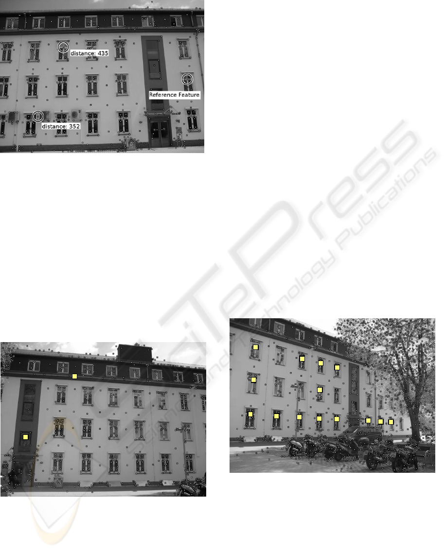
Figure 3: Euclidean distances between appropriate and ex-
ternal features.
SIFT features only by their Euclidean distances. In-
stead we have to develop other more sophisticated cri-
teria.
3.2 Scale and Orientation
SIFT is invariant in rotation and scale. This is essen-
tial in many applications with the goal to recognize
the same feature across different images which might
have been acquired after a change in the camera posi-
tion. But if only one image is relevant the invariance
attributes may become a hindrance.
Figure 4: Two features with a different semantics that are
similar in their 128-dimensional feature vector but different
in rotation.
Regard, e.g., a roof gutter. The invariance may
imply that a SIFT vector in a narrow black hori-
zontal roof gutter becomes similar to a vector in a
wide black vertical band on a building wall (compare
Fig.4). Both gradient patterns are similar but refer to
another scale and are rotated by 90
◦
. So, for group-
ing and distinguishing features correctly it is not suffi-
cient to only compare the feature vector, we also have
to compare the feature’s level of scale and its orienta-
tion.
Watching the scale of a feature it is possible to
gain fundamentalinformation. A big and a small quad
on a building wall cannot be distinguished by their
Euclidean distances. Using their value of scale it is
not a problem.
Similar advantages can be gained by using the fea-
ture orientation. The vectors of two similar features
where one is rotated by 180
◦
are mainly equal. Only
comparing their orientation makes it possible to dis-
tinguish the features.
However, if we compare all scale and orientation
of all features to the scale and orientation of the fea-
ture group’s start feature, new problems arise due to
perspective effects in the image. The following exam-
ple illustrates this: If one watches a line of windows
from a very angular view the windows get smaller in
vanishing point direction (Fig.5, the quads describe
features with a small Euclidean distance belonging
to the group of crossbars). As the windows size de-
creases the scale of the window describing features
also decreases. If we compare each features scale and
orientation to the scale and orientation of a larger win-
dow as reference feature the smaller windows would
be considered dissimilar.
Figure 5: Result of grouping algorithm in an image with
high angular perspective.
We approach this problem by averaging the dif-
ferences in scale and orientation over all processed
feature vectors which are already put into one feature
group. The threshold which determines whether the
difference in scale or orientation to the reference fea-
ture is acceptable is based on the respective mean dif-
ference. This ensures that the matching can adapt to
slightly varying scale or orientation due to e.g. per-
spective distortion.
VISAPP 2009 - International Conference on Computer Vision Theory and Applications
116

3.3 A Topology on SIFT Features
Incorporating scale and orientation helps us to distin-
guish visually dissimilar objects within similar SIFT
vectors. An other improvement of feature grouping
can be achieved by a more involved calculation of dis-
tance between two feature vectors.
Suppose a SIFT vector has in each of the 128
components a distance of 20 to the reference feature
resulting in an Euclidean distance of
√
128∗20
2
≃
226.3. Another one has a distance of 9 in all but ten
components and 60 in the other ten resulting in an
Euclidean distance of
√
118∗9
2
+ 10∗64
2
≃ 224.8.
However, our experiments show that few big differ-
ences are a stronger clue to different semantics than
many small differences.
We therefor don’t calculate the distance between
two feature vectors as the sum of all the 128 com-
ponent differences but as the sum of only the seven
largest component differences. We call this a 7-
distance. In the example above we would therefor
get the 7-distance
√
7∗20
2
≃52.9 for the many small
differences and
√
7∗64
2
≃ 169.3 for the few larger
differences.
Mathematically speaking, a SIFT feature f is a
tuple f = (s
f
, o
f
, v
f
, l
f
) of four attributes: s
f
for
the scale, o
f
for the orientation, v
f
for the 128-
dimensional vector, and l
f
for the location of the fea-
ture in x,y-coordinates in the image. The Euclidean
distance d
E
( f
1
, f
2
) and 7-distance d
7
( f
1
, f
2
) of two
SIFT features is the Euclidean and 7-distance between
v
f
1
and v
f
2
. The range of o
f
is [0, 2π]. The range
of s
f
depends on the size of the image and is about
0 ≤ i ≤ 100 in our examples.
We introduce a topology on SIFT features. For
this we say that f
′
= (s
′
, o
′
, v
′
, l
′
) belongs to the
(t
s
,t
o
,t
7
)-neighborhood of f = (s, o, v,l) if there
holds:
• |s−s
′
| < t
s
,
• |o−o
′
| < t
o
,
• d
7
( f, f
′
) < t
7
for three thresholds t
s
, t
o
, t
7
. Thus, the location
plays no role in this topology.
4 THE ALGORITHM
We now present the algorithm to build G( f), the
group of SIFT features generated by start feature f.
Let m
s
(G) and m
o
(G) be the mean differences in
scale and orientation of all SIFT features in a set G
with respect to f. Let f
i
denote the i-th closest SIFT
feature in the image to f with respect to d
E
.
1: G(f):={f}; i:=0; fault:=0;
2: t
s
:= 3.5; t
o
:= 1.0; t
7
:= 550
3: repeat
4: i:=i+1;
5: if f
i
belongs to the (t
s
,t
o
,t
7
)-neighborhood of f
and
(m
s
(G( f)) ≤ 0.5 or |s
f
−s
f
i
| ≤ 4·m
s
(G( f)))
and
(m
o
(G( f)) ≤0.01 or |o
f
−o
f
i
|≤10·m
o
(G( f))
then
6: G( f) := G( f) ∪{f
i
};
7: update m
s
(G( f));
8: update m
o
(G( f))
9: else
10: fault:=fault+1
11: end if
12: until fault=3
The chosen parameter t
s
depends on the size of the
image. It should be noted that the Euclidean distance
gives the candidates f
i
for G( f) while the 7-distance
d
7
excludes some of them. Both distances are thus
used.
5 RESULTS
For an evaluation we use examples from a database
of about 200 images of the campus of our Univer-
sity. These are 8 bit greyscale images of dimension
1024x768. The images have been acquired in differ-
ent weather conditions.
SIFT features which describe building character-
istics were chosen for analysis. The characteristics
analyzed in this paper are crossbars in windows (com-
pare Fig.6) and narrow windows (compare Fig.7).
Of course, what is essential is not a built group
G of features but their locations loc(G) in the image.
For a further image analysis the positions of similar
semantics in an image are important, not the features
used to find those positions. Due to rounding errors
the position of a feature in the discrete image may
vary. If we speak about the same position we just
mean a spatial distance of ≤ 1 pixel. There may be
in some rare cases two features f, f
′
at the same po-
sition with a very close Euclidean and 7-distance that
describe the same semantic object on different scales.
For such objects only that one with the larger group is
regarded in our evaluation analysis.
For all analyzed images the locations of those two
characteristics (crossbar, narrow window) have been
annotated by hand as ground truth. Only with such a
ground truth an quantitative evaluation becomes pos-
IMAGE UNDERSTANDING USING SELF-SIMILAR SIFT FEATURES
117

Figure 6: The characteristic crossbars are marked with cir-
cles.
Figure 7: The characteristic windows are marked with
points.
sible. Let G be a group resulting from our algorithm
in an image with a known ground truth GT. We mea-
sure the coverability rate CR(G, GT) and error rate
ER(G;GT):
CR(G, GT) :=
|loc(G) ∩GT|
|GT|
,
ER(G, GT) :=
|loc(G) −GT|
|G|
.
The coverability rate states how good the ground
truth locations were covered by G. The error rate
states how much of G is outside the ground truth.
The groupingresults differ in their quality depend-
ing on the chosen start feature. As a consequence,
we run the algorithm with every feature of the ground
truth as start feature. We then compute the mean CR
and ER of all computed groups.
5.1 Crossbar Analysis
We have analyzed 25 images for the crossbars. Those
images show buildings in different distances and an-
gles.
Table 1: Evaluation: Crossbars.
ID GT CR ER
min max mean min max mean
1 12 0.08 0.67 0.43 0.00 0.40 0.09
2 20 1.00 1.00 1.00 0.00 0.00 0.00
3 12 1.00 1.00 1.00 0.00 0.00 0.00
4 9 0.11 0.56 0.37 0.00 0.33 0.06
5 15 0.07 0.73 0.49 0.00 0.00 0.00
6 14 0.07 0.86 0.71 0.00 0.00 0.00
7 16 0.06 0.94 0.65 0.00 0.00 0.00
8 9 0.11 0.44 0.27 0.00 0.50 0.05
9 21 0.05 0.86 0.43 0.00 0.50 0.07
10 14 0.14 0.71 0.56 0.00 0.14 0.02
11 20 0.05 0.90 0.63 0.00 0.50 0.05
12 17 0.06 0.88 0.75 0.00 0.00 0.00
13 6 0.17 0.83 0.72 0.00 0.00 0.00
14 12 0.08 0.58 0.32 0.00 0.00 0.00
15 8 0.13 0.88 0.58 0.00 0.00 0.00
16 12 0.08 0.92 0.79 0.00 0.08 0.04
17 10 0.10 0.90 0.67 0.00 0.38 0.04
18 12 0.09 0.82 0.48 0.00 0.50 0.05
19 4 0.25 0.75 0.63 0.00 0.40 0.10
20 6 0.67 1.00 0.89 0.00 0.00 0.00
21 9 0.11 1.00 0.71 0.00 0.00 0.00
22 10 0.10 0.70 0.51 0.00 0.00 0.00
23 3 1.00 1.00 1.00 0.00 0.00 0.00
24 2 1.00 1.00 1.00 0.00 0.00 0.00
25 8 0.13 0.88 0.58 0.00 0.00 0.00
mean: 0.64 mean: 0.02
Table 1 shows that the average coverability rate
for all the images lies at 64% with a mean error rate
of 2%. Column GT tells how many feature positions
of that image belong to the ground truth. Only nearly
two-thirds of all the wanted features got grouped cor-
rectly by the algorithm. But there is high variance in
the results. The quality depends on the used start fea-
ture. For every start feature we get a fragment of the
correct feature group (See Fig.8 where we represent
the computed groups by quads). Interesting are im-
ages 2, 3, 23, and 24. In image 2 there are 20 feature
location in the ground truth. No matter with which
feature we start our algorithm always finds all loca-
tions correctly without any mistake.
In many images there is a maximum CR of 0.8
or higher. That means that there is the challenge to
identify and to use these maximum values correctly.
Extreme examples for different qualities are
shown in the figure 9, due to different start features.
VISAPP 2009 - International Conference on Computer Vision Theory and Applications
118

Figure 8: Two feature groups ”crossbar” with different start
features marked by a encircled star.
Figure 9: A good (16 members) and a very bad (just one
member) group due to different start features.
5.2 Narrow Window Analysis
We have evaluated 10 images for the narrow window
analysis. The images show the building in different
angles and under different weather conditions.
Table 2: Evaluation: Narrow windows.
ID GT CR ER
min max mean min max mean
1 27 0.59 1.00 0.95 0.00 0.00 0.00
2 28 0.04 0.96 0.84 0.00 0.50 0.01
3 23 0.04 0.91 0.73 0.00 0.06 0.00
4 28 0.04 1.00 0.80 0.00 0.00 0.00
5 14 0.07 1.00 0.76 0.00 0.00 0.00
6 25 0.08 0.96 0.85 0.00 0.00 0.00
7 19 0.16 1.00 0.83 0.00 0.57 0.06
8 11 0.09 0.90 0.62 0.00 0.00 0.00
9 26 0.04 0.88 0.72 0.00 0.33 0.02
10 28 0.04 0.96 0.84 0.00 0.50 0.15
mean: 0.79 mean: 0.03
The evaluation shows even better results than the
crossbar evaluation. The number of tested images is
not as big as the number of crossbar images but the
number of relevant features in the narrow window im-
ages is larger. The mean coverability rate of 79% with
an error rate of 3% is an acceptable result.
6 CONCLUSIONS
We have presented a new approach to identify seman-
tically similar objects by grouping SIFT features. As
SIFT was intended for matching between different
images we cannot just group SIFT features by their
Euclidean distance but have to considerate scale and
orientation differently.
Work on this approach is by no means completed.
On contrary, we see this as a start for an automatic
grouping of semantics. Besides obvious variants of
this algorithm worth to be investigated it is an inter-
esting task to compute a semantic group independent
of the chosen start feature. We will try to do this
by merging overlapping feature groups with different
start features.
REFERENCES
Bay, H., Tuytelaars, T., and Van Gool, A. (2006). Surf:
Speeded up robust features. In 9th European Confer-
ence on Computer Vision, Graz Austria.
Chum, O. and Matas, J. (2005). Matching with prosac -
progressive sample consensus. In CVPR (1), pages
220–226.
Fischler, M. and Bolles, R. (1987). Random sample con-
sensus: a paradigm for model fitting with applications
to image analysis and automated cartography. pages
726–740.
Goshen, L. and Shimshoni, I. (2006). Balanced exploration
and exploitation model search for efficient epipolar
geometry estimation. In ECCV06, pages II: 151–164.
Ke, Y. and Sukthankar, R. (2004). Pca-sift: A more distinc-
tive representation for local image descriptors.
Lowe, D. (1999). Object recognition from local scale-
invariant features. In Proc. of the International
Conference on Computer Vision ICCV, Corfu, pages
1150–1157.
Lowe, D. (2003). Distinctive image features from scale-
invariant keypoints. In International Journal of Com-
puter Vision, volume 20, pages 91–110.
Slot, K. and Kim, H. (2006). Keypoints derivation for object
class detection with sift algorithm. In Artificial Intel-
ligence and Soft Computing ICAISC 2006. Springer
Berlin , Heidelberg.
IMAGE UNDERSTANDING USING SELF-SIMILAR SIFT FEATURES
119