
PROJECTOR CALIBRATION USING A MARKERLESS PLANE
Jamil Drar
´
eni, S
´
ebastien Roy
DIRO, Universite de Montreal , CP 6128 succ Centre-Ville, Montreal QC, Canada
Peter Sturm
INRIA Rhone-Alpes , 655 Avenue de lEurope, 38330 Montbonnot St Martin, France
Keywords:
Video projector calibration, Planar calibration, Focal estimation, Structured light, Photometric stereo.
Abstract:
In this paper we address the problem of geometric video projector calibration using a markerless planar surface
(wall) and a partially calibrated camera. Instead of using control points to infer the camera-wall orientation,
we find such relation by efficiently sampling the hemisphere of possible orientations. This process is so fast
that even the focal of the camera can be estimated during the sampling process. Hence, physical grids and full
knowledge of camera parameters are no longer necessary to calibrate a video projector.
1 INTRODUCTION
With the recent advances in projection display, video
projectors (VP) are becoming the devices of choice
for active reconstruction systems. Such systems like
Structured Light (Salvi et al., 2004) and Photometric
Stereo (Woodham, 1978; Barsky and Petrou, 2003)
use VP to alleviate the difficult task of establishing
point correspondences. However, even if active sys-
tems can solve the matching problem, calibrated VP
are still required. In fact, a calibrated projector is
required to triangulate points in a camera-projector
structured light system, or to estimate the projector’s
orientation when the latter is used as an illuminant de-
vice for a photometric stereo system.
Since a video projector is often modeled as an in-
verse camera, it is natural to calibrate it as part of a
structured light system rather than as a stand alone
device. In order to simplify the calibration process, a
planar surface is often used as a projection surface on
which features or codified patterns are projected. The
projector can be calibrated as a regular camera, ex-
cept for the fact that a regular accessory camera must
be used to see the projector patterns. The way pat-
terns are codified and the projection surface orienta-
tion is estimated will distinguish the various calibra-
tion methods from each other.
In (Shen and Meng, 2002), a VP projects patterns
on a plane mounted on a mechanically controlled plat-
form. Thus, the orientation and position of the projec-
tion plane is known and is used to calibrate the struc-
tured light system using conventional camera calibra-
tion techniques.
Other approaches use a calibrated camera and a
planar calibration chessboard attached to the projec-
tion surface (Ouellet et al., 2008; Sadlo et al., 2005).
For convenience and because the projection sur-
face is usually planar, we will refer to it as the wall.
The attached chessboard is used to infer the orienta-
tion and the position of the wall w.r.t the camera. This
relation is then exploited, along with the images of the
projected patterns to estimate the intrinsic parameters
of the projector.
In order to measure the 3D position of the pro-
jected features, (Sadlo et al., 2005) estimates the ho-
mography between the attached chessboard and the
camera. This allows the computation of the extrin-
sic parameters of the camera. It is important to men-
tion that the camera must be fully calibrated in this
case. With at least three different orientations, a set
of 3D-2D correspondences can be obtained and then
used to estimate the VP parameters with standard
plane-based calibration methods (Sturm and May-
bank, 1999; Zhang, 1999). We refer to this method
as Direct Linear Calibration (DLC). To increase accu-
racy of the DLC, a printed planar target with circular
markers is used in (Ouellet et al., 2008), to calibrate
the camera as well as the projector.
In (Lee et al., 2004), a structured light system is
calibrated without using a camera. This is made pos-
377
DrarÃl’ni J., Roy S. and Sturm P.
PROJECTOR CALIBRATION USING A MARKERLESS PLANE.
DOI: 10.5220/0001559603770382
In Proceedings of the Fourth International Conference on Computer Vision Theory and Applications (VISIGRAPP 2009), page
ISBN: 978-989-8111-69-2
Copyright
c
2009 by SCITEPRESS – Science and Technology Publications, Lda. All rights reserved
sible by embedding light sensors in the target surface.
Gray-coded binary patterns are then projected to es-
timate the sensor locations and prewarp the image to
accurately fit the physical features of the projection
surface. The VP parameters are not explicitly esti-
mated but the method could easily be extended for
that purpose.
In this paper, a new projector calibration method
is introduced. The proposed method does not require
a physical calibration board nor a full knowledge of
the camera parameters.
We overcome the problem of determining the
camera-wall homography H
w→c
by exploring the
space of all acceptable homographies and consider
the one that minimizes the reprojection error (see
Figure.1). Since H
w→c
depends only on the orienta-
tion between the camera and the wall, the space of
acceptable homographies can be parameterized with
only 2 angles: the elevation and the azimuth angles
that define the normal vector at the wall.
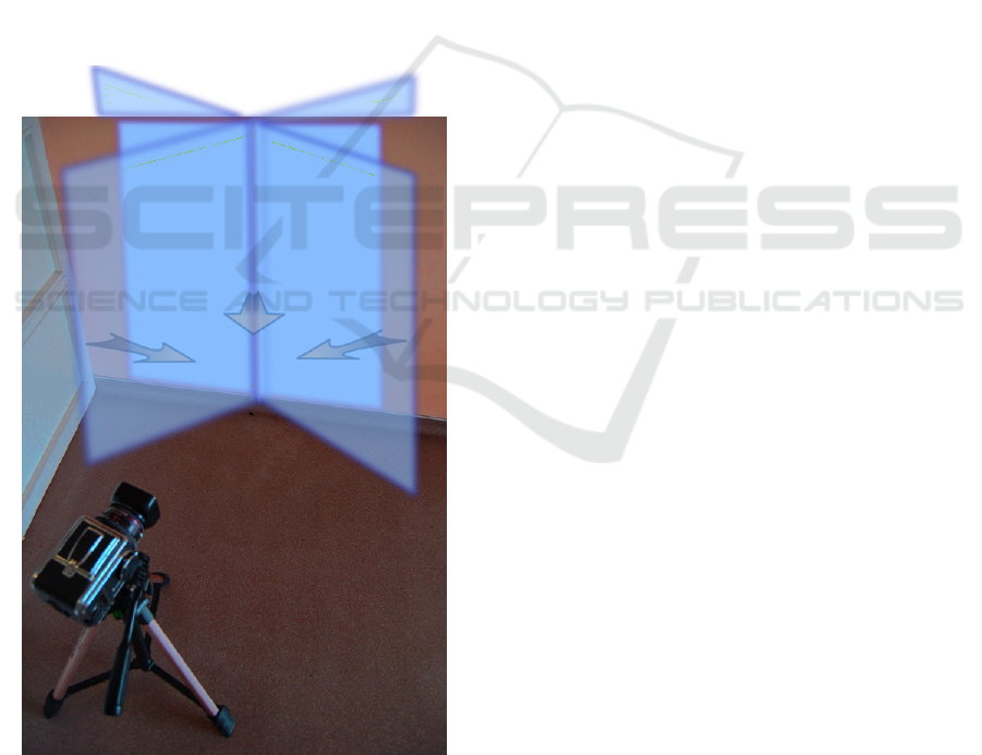
Figure 1: The homography wall-camera is defined by the
orientation of the wall.
Finding the normal of the wall consists then in
sampling the space of orientations on a unit sphere.
For each orientation sample, a DLC is performed and
we select the homography that minimizes the repro-
jection errors in the images. It is worth mentioning
that our DLC implementation differs slightly from the
one used in (Sadlo et al., 2005) as explained in the
next section.
Our proposed method is fully automatic, fast and
produces excellent results as shown in our experi-
ments. We also show that when the camera is not fully
calibrated, projector calibration is still tractable. This
is done by making the common assumptions that the
pixels are square and that the center of projection co-
incides with the image center (Snavely et al., 2006).
Thus, the only unknown camera parameter left to es-
timate is the focal length, which is estimated by sam-
pling.
The rest of this paper is organized as follows. Sec-
tion 3 presents our variant of the direct linear cali-
bration for a projector. Section 4 details our orien-
tation sampling calibration (OSC) using only a (par-
tially calibrated) camera and a marker-less projection
plane.
Section 5 presents the results of our calibration
method, followed by a discussion of limitations and
future work in Section 6.
2 VIDEO PROJECTOR MODEL
We model the video projector as an inverse camera.
Therefore, we intend to compute the intrinsic and ex-
trinsic parameters. Without loss of generality, we con-
sider in this paper a 4 parameters projector model,
namely: the focal length, the aspect ratio and the prin-
cipal point. Thus, the projector matrix K
p
is defined
as:
K
p
=
ρ f 0 cx
0 f cy
0 0 1
The extrinsic parameters that describe the i
th
pro-
jector pose are the usual rotation matrix R
i
and the
translation vector t
i
.
3 DIRECT LINEAR
CALIBRATION
In this section, we review the details of the Direct Lin-
ear Calibration for projectors. This method is used
as a reference for our benchmark test. As opposed
to (Sadlo et al., 2005), the variant presented here is
strictly based on homographies and does not require a
calibrated camera.
VISAPP 2009 - International Conference on Computer Vision Theory and Applications
378

If a static camera observes a planar surface (or a
wall), a homography is induced between the latter and
the camera image plane. This linear mapping (H
w→c
)
relates a point P
w
on the wall to a point P
c
in the cam-
era image as follows:
P
c
∼ H
w→c
· P
w
(1)
Where ∼ denotes equality up to a scale. Details
on homography estimation can be found in (Hartley
and Zisserman, 2004).
The video projector is used afterward to project
patterns while it is moved to various positions and
orientations. For a given projector pose i, correspon-
dences are established between the camera and the
VP, leading to a homography H
i
c→ p
. A point P
i
c
in
the image i is mapped into the projector as:
P
i
p
∼ H
c→ p
· P
i
c
(2)
Combining Eq.1 an Eq.2, a point P
w
on the wall is
mapped into the i
th
projector as:
P
i
p
∼ H
i
c→ p
· H
w→c
| {z }
H
i
w→ p
·P
w
(3)
On the other hand, P
i
p
and P
w
are related through
a perspective projection as:
P
i
p
∼ K
p
·
R
i
1
R
i
2
t
i
· P
w
(4)
Where K
p
, R
i
1,2
and t
i
are respectively the projec-
tor intrinsic parameters, the two first vectors of the ro-
tation matrix R
i
, and the translation vector. From Eq.3
and Eq.4, a relation between H
i
w→ p
and the extrinsic
parameters of the projector is derived as follows:
K
−1
p
· H
i
w→ p
∼
R
i
1
R
i
2
t
i
(5)
With at least two different orientations, one can
solve for K
−1
p
by exploiting the orthonormal prop-
erty of the rotation matrix as explained in (Sturm and
Maybank, 1999).
4 ORIENTATION SAMPLING
CALIBRATION
In this section we give the details of our proposed
video projector calibration method. As discussed ear-
lier, the justification for using an attached calibration
rig to the wall is to infer the homography wall-camera
in order to estimate the 3D coordinates of the pro-
jected features. We propose to estimate this wall-
camera relation by exploring the space of all possible
orientations since only the orientation of the wall w.r.t
the camera matters and not its position.
Another way to look at this orientation space is to
consider all vectors lying on a unit hemisphere placed
on the wall, as depicted on Figure 1.
The calibration process can be outlined in three
main steps:
• Pick a direction on the hemisphere.
• Compute the corresponding homography.
• Use the homography to perform a DLC calibra-
tion (Section 3).
The above steps are repeated for all possible di-
rections and the direction that minimizes the reprojec-
tion errors is selected as the correct plane orientation.
The first two steps are detailed in the next subsections.
The third one is straightforward from section 3.
4.1 Sampling a Hemisphere
The problem of exploring the set of possible orienta-
tions is dependent on the problem of generating uni-
formly distributed samples on the unit sphere (hemi-
sphere in our case).
Uniform sphere sampling strategies can be ran-
dom or deterministic (Yershova and LaValle, 2004).
The first class are based on random parameters gen-
eration, followed by an acceptance/rejection step de-
pending on whether the sample is or not on the
sphere. Deterministic methods produce valid samples
on a unit sphere from uniformly distributed parame-
ters, such method include (but not limited to) quater-
nion sampling (Horn, 1986), normal-deviate methods
(Knuth, 1997) and methods based on Archimedes the-
orem (Min-Zhi Shao, 1996). We chose to use the lat-
ter method for its simplicity and efficiency. As the
name suggests, this method is based on Archimedes
theorem on the sphere and cylinder which states that
the area of a sphere equals the area of every right
circular cylinder circumscribed about the sphere ex-
cluding the bases. This argument leads naturally to
a simple sphere sampling algorithm based on cylin-
der sampling (Min-Zhi Shao, 1996). Uniformly sam-
pling a cylinder can be done by uniformly choosing
an orientation θ
i
∈ [0,π] (we call it azimuth) to obtain
a directed vector d(θ
i
,0) (See Figure.2). After that,
a height h
i
is uniformly chosen in the range [−1,1].
The resulting vector, noted d
i
(θ
i
,h
i
), is axially pro-
jected on the unit sphere. According to the above the-
orem, if a point is uniformly chosen on a cylinder, its
inverse axial projection will be uniformly distributed
on the sphere as well, see (Min-Zhi Shao, 1996) for
further details.
In our case, we only need to sample the hemi-
sphere facing the camera. Thus the span of the
PROJECTOR CALIBRATION USING A MARKERLESS PLANE
379
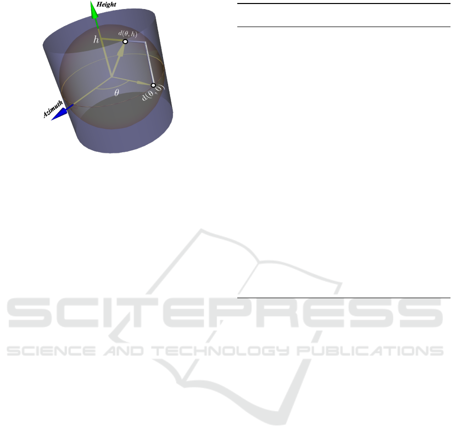
Figure 2: Orientation space sampling.
points that must be visited is limited to the range
[−1,+1]× [0,π].
4.2 Homography From an Orientation
Sample
The homography wall-camera H
i
w→c
induced by a
wall whose normal is a direction d
i
(as defined in the
previous subsection), is defined by:
H
i
w→c
∼ K
cam
.
R
i
1
R
i
2
t
(6)
Where K
cam
, R
i
1
, R
i
2
and t are respectively the in-
trinsic camera matrix, the first two vectors of the ro-
tation corresponding to the direction d
i
, and the trans-
lation vector. Without loss of generality and for the
sake of simplicity, we fix the projection of the origin
of the wall P
0
w
= (0,0)
T
into the camera at the image
center. With this convention, the translation vector t
simplifies to (0,0,1)
T
.
The rotation matrix R
i
is computed via Rodrigues
formula, which requires a rotation axis and a rota-
tion angle. The rotation axis is simply the result of
the cross product between d
i
and the vector (0,0,1)
T
whereas the rotation angle α
i
is obtained from the dot
product of the same vectors:
α
i
= cos
−1
d
i
T
· (0,0,1)
T
(7)
4.3 Complete Algorithm
We are now ready to give the complete algorithm
of our video projector calibration. We assume the
existence of two supporting functions, ReprojError
that returns a reprojection error for a given projector
parameters and DLC a function that estimate the
projector parameters using the DLC method (see
Section.3).
Algorithm 1: Orientation Sampling Calibra-
tion.
Data: H
k
c→ p
, the k camera-projector
homographies and K
cam
Camera intrinsic
matrix (optional).
foreach (h
i
,θ
i
)∈[−1,1]×[−π/2,π/2] do
Estimate direction d
i
(θ
i
,h
i
) (sec.4.1)
if K
cam
is undef then
Initialize elements of K
cam
using image
center and f
i
end
Estimate H
i
w→c
from d
i
and f
i
(sec.4.2)
foreach H
k
c→ p
do
H
k
w→ p
= H
k
c→ p
· H
i
w→c
end
K
i
pro j
← DLC(H
k
c→ p
) (sec.3)
Error ← ReprojError(K
i
pro j
)
if Error < BestError then
K
pro j
← K
i
pro j
BestError ← Error
end
end
return Projector calibration matrix K
pro j
5 EXPERIMENTS
We have evaluated the proposed calibration method
with both a calibrated and an uncalibrated cam-
eras. The results were also compared to the DLC
method. The evaluation platform consists of a Mit-
subishi pocket projector of 800 × 600 pixels resolu-
tion and a digital camera (Nikon D50). A 50mm lens
was used on the camera and the resolution was set
to 1500 × 1000. The calibration of the camera using
the Matlab toolbox gave the following intrinsic matrix
K
cam
:
K
cam
=
3176.3115 0 790.6186
0 3172.4809 495.3829
0 0 1
To include the DLC algorithm in our benchmark,
the camera was mounted on a tripod and was first reg-
istered to the wall using an attached printed chess-
board. Images of projected chessboard using the
video projector under several orientations were then
acquired using the camera. We took precaution to re-
move the attached chessboard form the wall before
acquiring the projector images to avoid overlaps be-
tween the projected patterns and the rigidly attached
pattern.
VISAPP 2009 - International Conference on Computer Vision Theory and Applications
380
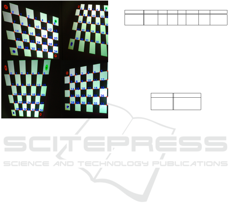
Some images of the projected chessboard along
with detected features are depicted on Figure.3.
Figure 3: Images of projected patterns and detected fea-
tures. The numbers and small red dots are added for illus-
tration only. The large dots in the 4 corners are part of the
projected pattern.
Notice the presence of colored dots on the chess-
board. Those were used to compute a rough esti-
mate of the homography (which will be refined) and
to eliminate the orientation ambiguity of the chess-
board while assigning 3D coordinates to the detected
features.
Our benchmark includes a projector calibration
using the DLC method, the proposed method with
both a calibrated and an uncalibrated camera. In the
first case, we used the image of the attached checker
to infer the wall-camera homography and calibrated
as explained in Section.3. For the second method,
we used a multi-resolution strategy to sample the az-
imuth angles and heights. The conditions of the third
method were identical to the second one except that
the camera parameters were ignored and were esti-
mated as follows:
• The focal length estimation was included in the
sampling process. The sampling range was
[0,10000].
• The pixels are assumed square.
• The center of projection is assumed to coincides
with the image center.
The result of this benchmark is outlined on the Ta-
ble.1. The table provides the estimated parameters,
Table 1: Projector calibration benchmark: Direct method,
Orientation sampling with a calibrated camera (Sampling-
C) and Orientation sampling with an uncalibrated camera
(Sampling-U).
Method f
proj
ρ cx cy estf
cam
Error Error B.A
Direct 1320.13 1.02 382.1 368 - 4.35 0.47
Sampling-C 1327.30 1.01 377.4 366 - 0.43 0.22
Sampling-U 1322.15 1.00 376 360 3108 0.16 0.09
the reprojection errors in pixels (Error), and the er-
ror difference comparing before and after applying a
bundle adjustment refinement (Error B.A). Technical
and implementation details on the latter can be found
in (Lourakis and Argyros, 2004).
The running times for a data set of 20 images on
an 1.5 Ghz computer are provided in Table.2.
Table 2: Execution time for Direct method, Sampling with
calibrated camera, and Sampling with uncalibrated camera.
Method Time (seconds)
Direct 0.18
Sampling-C 1.23
Sampling-U 6.2
From this test, we can see that our method, even
in the absence of camera parameters knowledge, out-
perform the Direct Linear Method at the expenses of a
higher running time. However, we are convinced that
the performance of our implementation could be fur-
ther improved by choosing a better multi-scale sam-
pling strategy. We also consider that not requiring a
printed chessboard attached to the wall is a major ad-
vantage, especially when the wall surface is large or
unaccessible.
A plot of the reprojection error in terms of the ori-
entation parameters h and α is provided in Figure.4.
We can clearly see that the function is very well be-
haved and easy to minimize.
As a last test, we wanted to assess the stability of
the focal length estimate. We thus fixed the value of
the wall orientation at the value obtained in the first
experiment and varied the focal length. The plot of
the reprojection error as a function of the sampled fo-
cal length of the camera is shown on Figure.5. As we
can see the error function is smooth and convex, sug-
gesting that the lack of knowledge of the focal length
can easily be circumvented in practice.
6 CONCLUSIONS
In this paper we presented a new video projector
calibration method. Contrary to most methods, we
showed that a physical target attached to a projection
surface is not necessary to achieve an accurate projec-
tor calibration. We also suggest that full knowledge
of camera parameters is not strictly required and can
PROJECTOR CALIBRATION USING A MARKERLESS PLANE
381
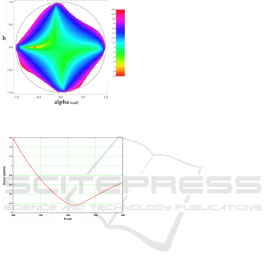
Figure 4: Reprojection error in terms of the orientation pa-
rameters h and α. The error computation does not include
bundle adjustment refinement.
Figure 5: Reprojection error in terms of the camera focal
length values (prior to bundle adjustment procedure). The
minimum is reached at 3034.4, the off-line camera calibra-
tion estimated a camera focal of 3176.
be relaxed into a set of commonly used assumptions
regarding the camera geometry. Very simple to im-
plement, the proposed method is fast and will handle
large projector-camera systems that were previously
impossible to calibrate due to the impractical chess-
board.
REFERENCES
Barsky, S. and Petrou, M. (2003). The 4-source photomet-
ric stereo technique for three-dimensional surfaces in
the presence of highlights and shadows. IEEE Trans-
actions on Pattern Analysis and Machine Intelligence,
25(10):1239–1252.
Hartley, R. I. and Zisserman, A. (2004). Multiple View Ge-
ometry in Computer Vision. Cambridge University
Press, ISBN: 0521540518, second edition.
Horn, B. K. P. (1986). Robot Vision (MIT Electrical Engi-
neering and Computer Science). The MIT Press, mit
press ed edition.
Knuth, D. E. (1997). Art of Computer Programming,
Volume 2: Seminumerical Algorithms (3rd Edition).
Addison-Wesley Professional.
Lee, J. C., Dietz, P. H., Maynes-Aminzade, D., Raskar, R.,
and Hudson, S. E. (2004). Automatic projector cali-
bration with embedded light sensors. In Proceedings
of the 17th annual ACM symposium on User interface
software and technology, pages 123–126. ACM.
Lourakis, M. and Argyros, A. (2004). The de-
sign and implementation of a generic sparse
bundle adjustment software package based on
the levenberg-marquardt algorithm. Technical
Report 340, Institute of Computer Science -
FORTH, Heraklion, Crete, Greece. Available from
http://www.ics.forth.gr/˜lourakis/sba.
Min-Zhi Shao, N. B. (1996). Spherical sampling by
archimedes’ theorem. Technical Report 184, Univer-
sity of Pennsylvania.
Ouellet, J.-N., Rochette, F., and H
´
ebert, P. (2008). Geo-
metric calibration of a structured light system using
circular control points. In 3D Data Processing, Visu-
alization and Transmission, pages 183–190.
Sadlo, F., Weyrich, T., Peikert, R., and Gross, M. (2005). A
practical structured light acquisition system for point-
based geometry and texture. In Proceedings of the
Eurographics Symposium on Point-Based Graphics,
pages 89–98.
Salvi, J., Pag
´
es, J., and Batlle, J. (2004). Pattern codifi-
cation strategies in structured light systems. Pattern
Recognition, 37(4):827–849.
Shen, T. and Meng, C. (2002). Digital projector calibration
for 3-d active vision systems. Journal of Manufactur-
ing Science and Engineering, 124(1):126–134.
Snavely, N., Seitz, S. M., and Szeliski, R. (2006). Photo
tourism: Exploring photo collections in 3d. In
SIGGRAPH Conference Proceedings, pages 835–846,
New York, NY, USA. ACM Press.
Sturm, P. and Maybank, S. (1999). On plane-based cam-
era calibration: A general algorithm, singularities, ap-
plications. In Proceedings of the IEEE Conference
on Computer Vision and Pattern Recognition, Fort
Collins, USA, pages 432–437.
Woodham, R. J. (1978). Photometric Stereo: A Reflectance
Map Technique for Determining Surface Orientation
from a Single View. In Proceedings of the 22
nd
SPIE
Annual Technical Symposium, volume 155, pages
136–143, San Diego, California, USA.
Yershova, A. and LaValle, S. M. (2004). Deterministic sam-
pling methods for spheres and so(3). In ICRA, pages
3974–3980.
Zhang, Z. (1999). Flexible camera calibration by viewing
a plane from unknown orientations. Computer Vision,
1999. The Proceedings of the Seventh IEEE Interna-
tional Conference on, 1:666–673 vol.1.
VISAPP 2009 - International Conference on Computer Vision Theory and Applications
382
