A SIMPLE METHOD OF CORTICAL BONE THICKNESS
EVALUATION BASED ON RADIOGRAPHIC IMAGES FOR
OSTEOPOROSIS INVESTIGATION
Przemysław Maćkowiak, Ryszard Stasiński
Department of Electronics and Telecommunications,Poznań University of Technology, Polanka 3, Poznań, Poland
Tomasz Kulczyk
Department of Biomaterials and Experimental Dentistry, Poznań University of Medical Sciences, Poland
Keywords: Osteoporosis population screening, Dental panoramic radiographs, Automatic bone borders extraction.
Abstract: In the paper a method of automatic extraction of cortical bone based on dental panoramic radiographs is
described. The method is intended for use as the first contact tool in osteoporosis population screening. Its
components have very low computational complexity, and can be found in every image processing software
package. The upper and lower boundaries of mandibular cortical bone have been determined in a series of
panoramic images, and results have been evaluated by a radiologist. The technique works either very
precisely, or clearly wrong (for heavily cluttered images), which proves its usefulness for an untrained user.
1 INTRODUCTION
Osteoporosis is a disease primarily affecting older
people, especially women aged over 60, and which
may lead to wrist, hip and vertebra fractures
(Torsoni et al., 2006). The modern gold standard for
evaluating osteoporosis is a BMD (Bone Mineral
Density) examination of the lumbar spine or/and
femoral neck. Currently access to a BMD
examination is limited as it is not possible to carry
out screening of all women over 65.
An alternative population screening test may be
based on the evaluation of certain parameters of
dental panoramic radiographs (Horner et al., 2002).
Dental panoramic images show the facial parts of
the skull with the upper and lower jaw and some
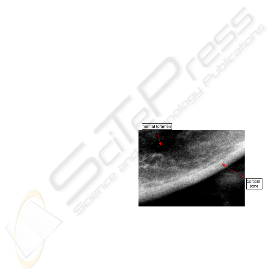
neighbouring structures. A particularly interesting
structure visible in a panoramic image is the cortical
bone of the lower border of mandible in the vicinity
of the mental foramen (Figure 1). Its parameters, e.g.
the width of the cortical bone and distance from the
lower border of the mandible to the mental foramen
can be measured as well as some characteristic
morphological features of the bone. If CW is below
3mm, an individual should be referred for the further
osteoporosis investigation (Horner et al., 2002).
Figure 1: Portion of a dental panoramic radiograph
showing the cortical bone and the mental foramen.
Analysis of morphological structures, in
conjunction with the results of measurements such
as PMI (Panoramic Mandibular Index), have been
correlated with data from a BMD test to investigate
any relationship between them. Some authors
believe that analysis of a panoramic image can result
in a dentist advising his patient to have a BMD test,
"because from your dental panoramic image it looks
as though you are in danger of osteoporosis” (Devlin
et al., 2007). The advantages of such a “screening
test“ are both economic and safe, since the
270
Ma
´
ckowiak P., Stasi
´
nski R. and Kulczyk T. (2009).
A SIMPLE METHOD OF CORTICAL BONE THICKNESS EVALUATION BASED ON RADIOGRAPHIC IMAGES FOR OSTEOPOROSIS INVESTIGA-
TION.
In Proceedings of the International Conference on Health Informatics, pages 270-275
DOI: 10.5220/0001549102700275
Copyright
c
SciTePress
panoramic image has already been taken for other
purposes and the patient is not subject to additional
radiation. Such a test should be automated, as
evaluations done by general dental practitioners may
differ importantly from those given by radiologists
(Devlin et al., 2001).
Currently it exists only few works on automatic
analysis of panoramic images for osteoporosis
examination, and the based on active contours
(snakes) method from paper (Devlin et al., 2007)
requires specialised software. This article presents a
computer algorithm consisting of simple and
readibly available components, which seems to
provide reliable measurements of the cortical bone.
The article is divided as follows. Chapter two
describes the research material. Third chapter is the
algorithm description. The fourth and the fifth
chapter are the discussion and the results. The last
ones are the conclusions and the literature.
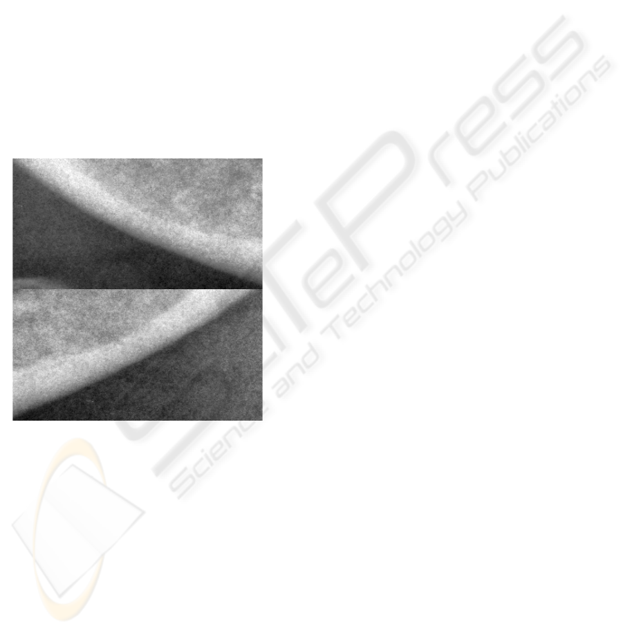
Figure 2: The region of interests for the right and left sides
of a panoramic radiograph at the mandible.
2 RESEARCH MATERIAL
40 digital dental panoramic images have been taken
using the CRANEX TOME dental panoramic unit
and a DIGORA PCT PSP DIGITAL SCANNER.
Images of 3258x1764 resolution have been provided
by the Section of Dental Radiology in the
Department of Biomaterials and Experimental
Dentistry, Poznań University of Medical Sciences.
Two small parts of the image from the left and right
sides were cut off by the radiologist to create regions
of interest (ROI) for further analysis. Each ROI has
had a rectangular shape and has contained the region
extending from edge of mental foramen down to and
below the lower edge of cortical bone, as illustrated
in Figure 2. The size of the ROI may vary but must
include the region around the mental foramen and
extend below the lower border of mandible.
3 ALGORITHM DESCRIPTION
The goal is to determine the upper and lower
boundaries of the cortical bone accurately. This task
requires generation of two images, A and B,
specified in sections 3.1 and 3.2. The images are
inputs to a contour extraction method described in
section 3.3, leading to determination of the desired
boundaries. The algorithm is based on linear and
morphological filtering.
The algorithm has been tested for images having
fixed resolution. For other resolutions different mask
sizes (M1 and M2, defined below) should be applied
when low-pass and high-pass filtering an image.
3.1 Image A
Image A provides the upper boundary of the cortical
bone. The algorithm consists of six steps; input
image is the ROI cut:
High-pass filtering (M1 mask),
Low-pass filtering (M1 mask), twice,
Image brightness normalization,
Thresholding
Selection of the biggest object.
3.1.1 High-pass and Low-pass Filtering
A signal can be treated as the sum of low-pass and
high-pass components. Using this observation, high-
pass filtering can be done as follows:
J = I – LOWPASS(I, M1), (1)
where I is the original image, LOWPASS(I,M1)
means low-pass filtering of image I using mask M1.
The M1 mask is the matrix of 31x31 elements equal
to 1/31
2
, and has a notch filter characteristic.
Image J is low-pass filtered using the same mask
M1, the operation is performed twice. It leads to
boundary adjustment (less roughness), but some
blurring, which is corrected in next steps. The use of
a too small mask leads to important roughness of
boundaries after thresholding operation. Of course,
double low-pass filtering can be replaced by a single
one at the expense of increased computational time.
A SIMPLE METHOD OF CORTICAL BONE THICKNESS EVALUATION BASED ON RADIOGRAPHIC IMAGES
FOR OSTEOPOROSIS INVESTIGATION
271
3.1.2 Brightness Normalization
The next processing step relies on image brightness
normalization. 5th and 95th percentiles of image
histogram are computed and the L and H thresholds
are obtained. Pixels are assigned an intensity of zero
or one (maximum) if their brightness is below or
above thresholds L and H respectively. If the pixel
intensity is between L and H, a new pixel brightness
score is assigned according to the equation
()
L-y)IN(x,
L-H
1
y)OUT(x, ⋅=
, (2)
where OUT is the output image, IN describes the
input image, (x,y) are a pair of coordinates. This is a
simple linear transformation which leads to contrast
improvement in the interval <L,H>.
3.1.3 Thresholding
Only one global threshold is used, as experiments
have shown good results have been obtained for
threshold values T = 175/255 or T = 180/255. It
should be emphasized that more accurate boundary
determination is ensured for a variable threshold, but
the algorithm is not fully automatic in such case.
Image thresholding based solely on highpass
filtering (one global threshold) doesn’t give good
results, as artifacts tend to appear (many twigs). In
such cases upper boundary extraction is difficult.
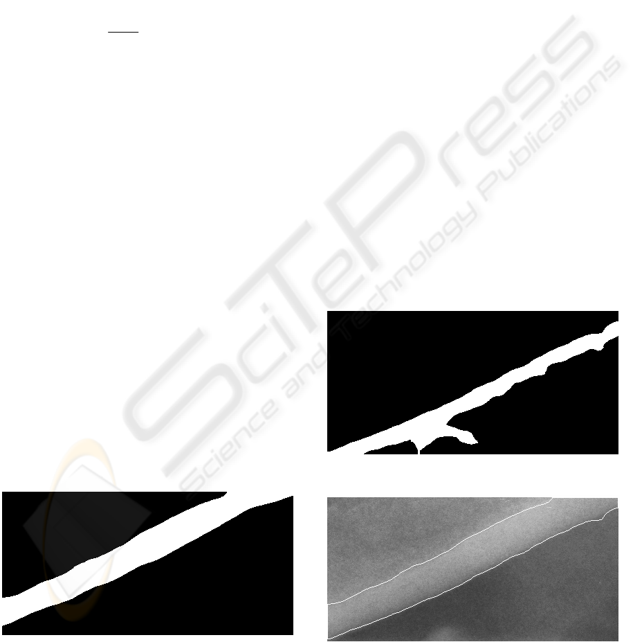
3.1.4 Selection of the Biggest Object
At this point the (binary) image contains many small
structures, so the next step is to erase all objects but
the one with the biggest surface (structures surfaces
should be computed). An example is presented in
figure 3. Upper part of its contour is the desired
boundary to be extracted.
Figure 3: Example of image A.
3.2 Image B
Image B provides the lower boundary of the cortical
bone. It is much better visible than the upper one, as
the lower boundary occurs in the region of greater
contrast. The algorithm consists of six steps:
• Opening (mask 5x5),
• Low-pass filtering (mask M2),
• High-pass filtering (mask M1),
• Image brightness normalization,
• Thresholding,
• Selection of the biggest object.
Initially the opening operation is carried out
using a 5x5 window (all its elements equal to one),
which involves two nonlinear filtering steps: a
minimum filtering and a maximum filtering. A low-
pass filtering mask M2 consists of 21x21 elements
each having the value 1/21
2
. At this stage the image
is blurred. High-pass filtering, which is the next step,
emphasizes brightness differences and involves the
use of the previously defined M1 mask. The image
normalization stage has been described in section
3.1.2. Thresholding is performed using a global
threshold T2 equal to 0.35, as a result a binary image
is received. The biggest object is selected in the next
step, its upper limit is the lower cortical bone
boundary. A result is shown in figure 4.
Figure 4: Example of image B (same case as in figure 3).
Figure 5: Boundaries from Figures 3 and 4 superimposed
on the original image.
HEALTHINF 2009 - International Conference on Health Informatics
272

3.3 Contour Extraction
The algorithm combines boundaries of images A and
B. An exemplary result is shown in figure 5.
A and B images are inputs to the contour
extraction method. RESULT is the result image,
additionally, TEMP_TAB and POINTS tables are
used, k and j are indices; at the beginning k and j
equal one, while RESULT, TEMP_TAB contain
zeros. The size of the RESULT image is the same
and equal the size of the A image. The size of the
TEMP_TAB equals the column number of the image
A, the size of the POINTS table equals zero or one.
LAST is the variable determing the number of
column of image A.
1. Find the first white pixel in the k-th column in
the image A (searching is done from the last
row to the first one).
2. Find the first white pixel in the k-th column in
the image B (searching is done from the first
row to the last one).
3. If both pixels are found, execute the following
tasks and go to step 7: join them by the shortest
path (set of white pixels along the k-th column),
mark the connection in the image A (put white
pixel), TEMP_TAB[k]=1, check if the
difference between TEMP_TAB[k] and
TEMP_TAB[k-1] equals one, if it does, put
current k value to the table POINTS.
4. If none of pixels is found, go to step 7.
5. If the white pixel from the image B is not found
and the white pixel from image A is found,
execute following tasks and go to the step 7:
find the first white pixel in the k-th column of
the image A (searching is done from the first
row to the last row), remove all white pixels
from column k (put black pixels), with the
exception of the first white pixel found.
6. If the white pixel from the image B is found and
the white pixel for the image A is not found,
mark it in the A image (put white pixel) and
continue (go to step 7).
7. k = k +1, if k≤LAST, go to step 1, otherwise
continue.
8. Fill any holes in the image A.
9. Create RESULT image by extracting perimeter
of image A (RESULT= PERIMETER(A)).
10. Find all indices {m} for which TEMP_TAB[m]
– TEMP_TAB[m-1] equals -1, put them to the
separate cells of the POINTS table, if the size of
the POINTS table is greater than zero, go to the
next step, otherwise stop the algorithm.
11. Find the first white pixels in the POINTS[j]-th
column from the bottom and from the top of the
image.
12. Assign zero values in the RESULT image to the
pixels between pixels found (along the
POINTS[j]-th column), j = j +1, if j is greater
than the size of POINTS table, stop the
algorithm, otherwise go to step 11.
The flowgraph of the contour extraction algorithm is
shown in figure 6.
4 RESULTS
Forty images have been tested. The cortical bone
contours were extracted. Thresholds T=175/255 and
T=180/255 were used for the right and left side of
the dental panoramic radiograph respectively (image
A). The resulting boundaries have been presented to
a radiologist for verification and have been either
accepted or rejected. There is an irremovable
element of subjectivity in such a test, boundaries
sketched by a human aren’t absolutely strict, and
differ slightly from an evaluation session to another
one.
Table 1: The upper boundary, the left side.
Clutter free (N=28) Cluttered (N=12)
Accepted 26 Accepted 4
Rejected 2 Rejected 8
Table 2: The lower boundary, the left side.
Clutter free (N=28) Cluttered (N=12)
Accepted 28 Accepted 8
Rejected 0 Rejected 4
Table 3: The upper boundary, the right side.
Clutter free (N=31) Cluttered (N=9)
Accepted 30 Accepted 4
Rejected 1 Rejected 5
Table 4: The lower boundary, the right side
Clutter free (N=31) Cluttered (N=9)
Accepted 31 Accepted 5
Rejected 0 Rejected 4
Tables 1, 2 and 3, 4 present verification results
concerning the upper and lower cortical bone
boundaries for the left and right side, respectively.
Images have been classified either as cluttered or
clutter free. The cluttered images contain structures
which overlap the upper or lower cortical bone.
A SIMPLE METHOD OF CORTICAL BONE THICKNESS EVALUATION BASED ON RADIOGRAPHIC IMAGES
FOR OSTEOPOROSIS INVESTIGATION
273

There have been 12 and 9 images in which other
structures overlapped left or right side of DPR,
respectively.
As can be seen, in the case of clutter-free images
the results for extraction of cortical bone boundaries
have been from very good (26 correct ones out of 28
possible for upper boundary, left side) to perfect
ones (both lower boundaries). In contrast, results for
cluttered images are rather poor. Note however that
such images are easily discernible from the clutter-
free ones. Moreover, whenever the method have
failed, it has been very clear even for a non-
specialist that the extracted boundaries did not
define the cortical bone.
The particularly good results for the lower
cortical bone extraction result from higher contrast
at the edge of cortical bone. In the region of the
upper boundary of cortical bone the contrast is
usually much lower due to the presence of spongy
bone. In some cases when positioning of the patient
during x-ray examination was not performed
correctly, the superimposition over the upper cortical
boundary of other anatomical structures such as
hyoid bone was observed in the form of "clutter". In
a few cases the exact location of the upper cortical
border was uncertain even to the radiologist due to
factors mentioned above.
When comparing with existing methods (Devlin
et al., 2007) note that the algorithm presented is
neither complex nor a time consuming one. Firstly,
in contrast to the method based on snakes it is non-
iterative, results are obtained in a single run. Time
complexity of each of its steps is O(n), i.e. the
smallest possible. The prototype function written in
MATLAB (version 7.0) realizing the algorithm
executed in 0.4s for one image on 1.6 GHz Intel
Celeron with 1GB RAM, an optimized program
would be an order of magnitude faster. The snakes
are moving across an image, the computation of a
dislocation for each segment of a snake requires
solving some equilibrium equations. Of course, it
might be done quite time-effectively, if precision
need not be high. Unfortunately, the method from
(Devlin et al., 2007) forms a basis for a commercial
software, hence, the details are not known.
When image contains structures that overlap the
upper cortical bone, thresholding often do not lead to
correct extraction. Note, however that unless a
method has a human-like ability to draw a known
shape on the basis of its small fraction, correct bone
extraction in heavily cluttered images is a hopeless
task. Straightforward use of snakes does not
guarantee the success, too. That is why a clearly
wrong outline of a cortical bone in such images
seems to be a much better result than a shape that is
probable, but highly imprecise one.
6 CONCLUSIONS
A new simple and effective algorithm for extracting
cortical bone boundaries has been described in the
paper. It consists of elementary operations available
as functions in every image processing software
package. The method works very well for clutter-
free images, on the other hand, it is very clear when
it fails in cases when the image is highly misleading.
This combination of features is ideal for an
untrained algorithm user, hence, the method is an
excellent auxiliary tool for osteoporosis
investigation by general dentist practitioners.
As it has been mentioned in the introduction, the
proposed algorithm can be used for the cortical bone
width determination, which seems to be useful for
identification of women with low BMD level (Arifin
A. et al., 2006). Future work will be concentrated on
automatic cortical bone width measurement based
on the proposed algorithm.
REFERENCES
Tosoni, G.M., Lurie, A.G., Cowan, A.E., Burleson, J.A.,
2006. Pixel intensity and fractal analyses detecting
osteoporosis in perimenopausal and postmenopausal
women by using digital panoramic images. In Oral
Surgery, Oral Medicine, Oral Pathology, Oral
Radiology, and Endodontics. Vol. 102(2), pp. 235-
241.
Horner K., Devlin H., Harvey L., 2002. Detecting patients
with low skeletal bone mass. In J. Dent. Vol. 30, pp.
171-175.
Devlin H., Allen P.D., Graham J., Jacobs R., Karayianni
K., Lindh C., van der Stel P.F., Harrison E., Adams
J.E., Pavitt S., Horner K., 2007. Automated
osteoporosis risk assessment by dentists: A new
pathway to diagnosis. In Bone. Vol. 40, pp. 835–842.
Devlin C.V., Horner K., Devlin H., 2001. Variability in
measurement of radiomorphometric indices by general
dental practitioners. In Dentomaxillofac Radiol. Vol.
30, pp. 120-125.
Arifin A. Z.,Asano A., Taguchi A., Nakamoto T., Ohtsuka
M., Truda M., Kudo Y., Tanimoto K., 2006.
Computer-aided system for measuring the mandibular
cortical width on dental panoramic radiographs in
identifying postmenopausal women with low bone
mineral density. In Osteoporosis International, Vol.
17, pp. 753–759.
HEALTHINF 2009 - International Conference on Health Informatics
274
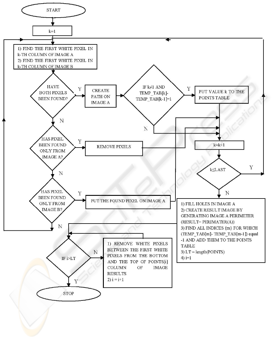
Figure 6: The flowchart of the contour extraction method.
A SIMPLE METHOD OF CORTICAL BONE THICKNESS EVALUATION BASED ON RADIOGRAPHIC IMAGES
FOR OSTEOPOROSIS INVESTIGATION
275
