3D RECONSTRUCTION FOR TEXTURELESS SURFACES

Surface Reconstruction for Biological Research of Bryophyte Canopies

Michal Krumnikl, Eduard Sojka, Jan Gaura

Department of Computer Science, V

SB - Technical University of Ostrava, 17. listopadu 15/2172, Ostrava, Czech Republic

Old

rich Motyka

Institute of Environmental Engineering, V

SB - Technical University of Ostrava

17. listopadu 15/2172, Ostrava, Czech Republic

Keywords:

3D reconstruction, Camera calibration, Depth from focus, Depth from illumination, Bryophyte canopy, Sur-

face roughness.

Abstract:

This paper covers the topic of three dimensional reconstruction of small textureless formations usually found

in biological samples. Generally used reconstructing algorithms do not provide sufﬁcient accuracy for sur-

face analysis. In order to achieve better results, combined strategy was developed, linking stereo matching

algorithms with monocular depth cues such as depth from focus and depth from illumination.

Proposed approach is practically tested on bryophyte canopy structure. Recent studies concerning bryophyte

structure applied various modern, computer analysis methods for determining moss layer characteristics draw-

ing on the outcomes of a previous research on surface of soil. In contrast to active methods, this method is a

non-contact passive, therefore, it does not emit any kind of radiation which can lead to interference with moss

photosynthetic pigments, nor does it affect the structure of its layer. This makes it much more suitable for

usage in natural environment.

1 INTRODUCTION

Computer vision is still facing the problem of

three-dimensional scene reconstruction from two-

dimensional images. Not a few algorithms have been

developed and published to solve this problem. These

algorithms can be divided into two categories; passive

and active (Jarvis, 1983). Passive approaches such as

shape from shading or shape from texture recover the

depth information from a single image (Horn, 1986;

Horn and Brooks, 1986; Coleman and Jain, 1981;

Prados and Faugeras, 2005). Stereo and motion anal-

ysis use multiple images for ﬁnding the object depth

dependencies (Ogale and Aloimonos, 2005; Kanade

and Okutomi, 1994; Sun et al., 2005; Kolmogorov

and Zabih, 2001). These algorithms are still devel-

oped to achieve higher accuracy and faster computa-

tion, but it is obvious that none will ever provide uni-

versal approach applicable for all possible scenes.

In this paper, we present combined strategy for re-

constructing three dimensional surface of textureless

formations. Such formations can be found in biologi-

cal and geological samples. Standing approaches suf-

fer mainly from the following shortcomings: high er-

ror rate of stereo correspondence in images with large

disparities, feature tracking is not always feasible,

samples might be damaged by active illumination sys-

tem, moreover biological samples can even absorb in-

cident light. Observing these drawbacks we have de-

veloped system linking several techniques, specially

suited for our problem.

Presented reconstruction method was tested on

bryophyte canopies surfaces. Obtaining three dimen-

sional surface is the ﬁrst stage of acquiring surface

roughness, which is used as biological monitor (Rice

et al., 2005; Motyka et al., 2008).

2 METHODS

In this section we will brieﬂy describe the methods

involved in our system, emphasizing improvements to

increase the accuracy and the density of reconstructed

points. As the base point, stereo reconstruction was

chosen. Selected points from the reconstruction were

used as the reference points for depth from illumina-

Krumnikl M., Sojka E., Gaura J. and Motyka O. (2009).

3D RECONSTRUCTION FOR TEXTURELESS SURFACES - Surface Reconstruction for Biological Research of Bryophyte Canopies.

In Proceedings of the International Conference on Bio-inspired Systems and Signal Processing, pages 95-100

DOI: 10.5220/0001539400950100

 SciTePress

tion estimation. Missing points in the stereo recon-

struction were calculated from the illumination and

depth from focus estimation. The last technique pro-

vides only rough estimation and is largely used for the

veriﬁcation purposes.

2.1 Stereo 3D Reconstruction

The following main steps leading to a reconstruction

of a sample surface are performed by particular parts

of the system: (i) calibration of the optical system

(i.e., the pair of cameras), (ii) 3D reconstruction of

the sample surface itself. In the sequel, the mentioned

steps will be described in more details.

In the calibration step, the parameters of the opti-

cal system are determined, which includes determin-

ing the intrinsic parameters of both the cameras (focal

length, position of the principal point, coefﬁcients of

nonlinear distortion of the lenses) and the extrinsic pa-

rameters of the camera pair (the vector of translations

and the vector of rotation angles between the cam-

eras). For calibrating, the chessboard calibration pat-

tern is used. The calibration is carried out in the fol-

lowing four steps: (1) creating and managing the set

of calibration images (pairs of the images of calibra-

tion patterns captured by the cameras), (2) processing

the images of calibration patterns (ﬁnding the chess-

board calibration pattern and the particular calibration

points in it), (3) preliminary estimation of the intrin-

sic and the extrinsic parameters of the cameras, (4) ﬁ-

nal iterative solution of all the calibration parameters.

Typically, the calibration is done only from time to

time and not necessarily at the place of measurement.

For solving the tasks that are included in Step 2,

we have developed our own methods that work au-

tomatically. For the initial estimation of the parame-

ters (Step 3), the method proposed by Zhang (Zhang,

1999; Zhang, 2000) was used (similar methods may

now be regarded as classical; they are also mentioned,

e.g., by Heikilla and Silven (Heikilla and Silven,

1997), Heikilla (Heikilla, 2000), Bouguet (Bouguet,

2005) and others). The ﬁnal solution of calibration

was done by the minimization approach. The sum of

the squares of the distances between the theoretical

and the real projections of the calibration points was

minimized by the Levenberg-Marquardt method.

If the optical system has been calibrated, the sur-

face of the observed sample may be reconstructed,

which is done in the following four steps: (i) captur-

ing a pair of images of the sample, (ii) correction of

geometrical distortion in the images, (iii) rectiﬁcation

of the images, (iv) stereomatching, (v) reconstruction

of the sample surface.

Distortion correction removes the geometrical dis-

tortion of the camera lenses. The polynomial distor-

tion model with the polynomial of the sixth degree is

used. The distortion coefﬁcients are determined dur-

ing the calibration.

Rectiﬁcation of the images is a computational step

in which both the images that are used for reconstruc-

tion are transformed to the images that would be ob-

tained in the case that the optical axes of both cameras

were parallel. The rectiﬁcation step makes it easier to

solve the subsequent step of ﬁnding the stereo corre-

spondence, which is generally difﬁcult. The rectiﬁca-

tion step is needed since it is impossible to guarantee

that optical axes are parallel in reality. We have devel-

oped a rectiﬁcation algorithm that takes the original

projection matrices of the cameras determined during

calibration and computes two new projection matri-

ces of ﬁctitious cameras whose optical axes are par-

allel and the projection planes are coplanar. After the

rectiﬁcation, the corresponding points in both images

have the same y-coordinate.

The dense stereo matching problem consists of

ﬁnding a unique mapping between the points be-

longing to two images of the same scene. We say

that two points from different images correspond one

to another if they depict a unique point of a three-

dimensional scene. As a result of ﬁnding the corre-

spondence, so called disparity map is obtained. For

each image point in one image, the disparity map con-

tains the difference of the x-coordinates of that point

and the corresponding point in the second image. The

situation for ﬁnding the correspondence automatically

is quite difﬁcult in the given context since the struc-

ture of the samples is quite irregular and, in a sense,

similar to noise. We have tested several known al-

gorithms (Kolmogorov and Zabih, 2001; Kanade and

Okutomi, 1994; Ogale and Aloimonos, 2005) for this

purpose. The results of none of them, however, are

fully satisfactory for the purpose of reconstruction.

Finally, we have decided to use the algorithm that was

proposed by Ogale and Aloimonos (Ogale and Aloi-

monos, 2005) that gave the best results in our tests.

2.2 Auxiliary Depth Estimators

The depth map obtained from the 3D reconstruction

is further processed in order to increase the resolu-

tion and ﬁll the gaps of missing data. To achieve this

we have implemented several procedures based on

the theory of human monocular and binocular depth

perception (Howard and Rogers, 1996). Exploited

monoculars cues were depth from the focus and light-

ing cues.

Depth estimation based on lighting cues was pre-

sented in several papers (Liao et al., 2007; Magda

BIOSIGNALS 2009 - International Conference on Bio-inspired Systems and Signal Processing

et al., 2001; Ortiz and Oliver, 2000). Methods pro-

posed in these papers were stand-alone algorithms re-

quiring either calibrated camera or controlled light

source. More simpliﬁed setup was proposed in (Liao

et al., 2007) using projector mounted on a linear stage

as a light source. These approaches calculate depth

from multiple images taken from different angles or

with varying lighting.

For our application we have developed slightly

modiﬁed method based on the previous research

which is capable of acquiring depths from just one

image. Assuming that we have already preliminary

depth map (e.g. disparity map from the stereo match-

ing algorithm) we can ﬁnd the correspondence of

depth and the light intensity.

According to the inverse square law, the measured

luminous ﬂux density from a point light source is in-

versely proportional to the square of the distance from

the source. The intensity of light I at distance r is

I =

4πr

, I ∝

, here P is the total radiated power

from the light source. Analyzed surfaces were ap-

proximated by Lambertian reﬂectors.

In contrast to (Liao et al., 2007) we are assuming

mostly homogeneous textureless uniform colored sur-

faces. Observing these assumptions we can omit the

step involving the computation of the ratio of inten-

sity from two images and alter the equation in order

to exploit already known depth estimation from pre-

vious 3D reconstruction based on the stereo matching

algorithm. Points that show high level of accuracy in

the previous step are used as the reference points for

illumination estimation. Look-up table, based on the

inverse square law, mapping the computed depth to

intensity is calculated.

The last method involved in the reconstruc-

tion step is the integration of focus measurement.

The depth from focus approaches have been used

many times for real time depth sensors in robotics

(Wedekind, 2002; Chaudhuri et al., 1999; Nayar et al.,

1996; Xiong and Shafer, 1993). Key to determine

the depth from focus is the relationship between fo-

cused and defocused images. Blurring is represented

in the frequency domain as the low-pass ﬁlter. The fo-

cus measure is estimated by frequency analysis. Dis-

crete Laplacian is used as the focus operator. For each

image segment, depth is estimated as the maximal

output of the focus operator. Since the images were

taken from short range, the lens focus depth was large

enough to capture the scene with high details. Thus

only a few focus steps were used in the experiments.

The ﬁnal depth is calculated as the weighted av-

erage from values given by stereo reconstruction pro-

cess, light intensity and depth from focus estimation.

Appropriate weights were set according to the exper-

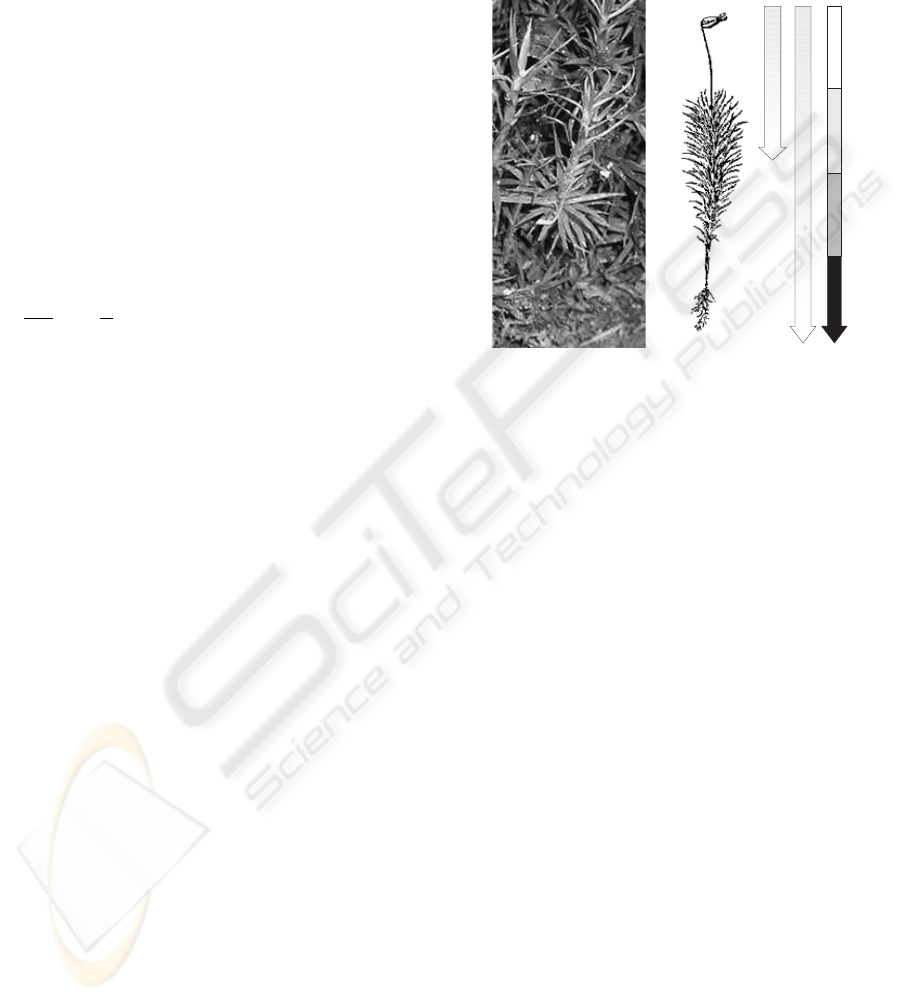
imental results gained with each method. The graphi-

cal illustration (Figure 1) shows the depth of acquired

data. Still the biggest disadvantage of camera based

scanning technique is the occurrence of occlusions,

decreasing the reconstructed point density.

STEREOVISION

PHOTOMETRY

FOCUS

Figure 1: Comparison of Used Methods for Depth Estima-

tion.

3 BRYOPHYTE STRUCTURE

Bryophytes are plants of a rather simple structure,

they lack of roots and conductive tissues of any kind

or even structural molecules that would allow es-

tablishment of their elements such as lignin (Crum,

2001). The water which is generally needed for

metabolic processes including photosynthesis is in the

case of bryophytes also necessary for reproductive

purposes, for their spermatozoids, particles of sexual

reproduction, are unable to survive under dry condi-

tions (Brodie, 1951). This makes them, unlike tra-

cheophytes (vascular plants), poikilohydric – strongly

dependent on the water conditions of their vicinity

(Proctor and Tuba, 2002) – which led to several eco-

logical adaptations of them. One of the most impor-

tant adaptations is forming of a canopy – more or less

compact layer of moss plants, frequently of a same

clonal origin, which enables the plants to share and

store water on higher, community level.

Recent infrequent studies concerning bryophyte

canopy structure applied various modern, computer

analysis methods to determine moss layer characteris-

tics drawing on the outcomes of a research on surface

of soil (Darboux and Huang, 2003). Surface rough-

ness index (L

) has been hereby used as a monitor of

quality and condition of moss layer, other indices, i.e.

the scale of roughness elements (S

) and the fractal di-

mension (D) of the canopy proﬁle have been used and

3D RECONSTRUCTION FOR TEXTURELESS SURFACES - Surface Reconstruction for Biological Research of

Bryophyte Canopies

found to be important as well (Rice et al., 2001). As

stated in Rice (Rice et al., 2005), contact probe, LED

scanner and 3D laser scanner were used and com-

pared in light of efﬁciency and serviceability in 27

canopies of different growth forms. However, none of

the methods already assessed have not been found to

be convenient for ﬁeld research, especially due to the

immobility of used equipment and therefore needed

dislocation of the surveyed moss material into the lab-

oratory. This has great disadvantage in destroying the

original canopy not only due to the transfer and ex-

cision from its environment, but also due to different

much dryer conditions affecting moss surface in lab-

oratory.

4 BRYOPHYTE CANOPY

ANALYSIS

The former methods (Rice et al., 2001; Rice et al.,

2005) are suitable and efﬁcient for measuring struc-

tural parameters in laboratory, but generally are im-

practicable in the ﬁeld. Despite the LED scanner is

presented as a portable device, it has high demands

for proper settings and conditions that has to be main-

tained.

The method described in this paper presents a new

approach using the pair of cameras as the scanning de-

vice. Computer analysis involving 3D reconstruction

and soil roughness compensation is used to calculate

the canopy surface roughness. The main goal was to

create a device that can be used in the ﬁeld, needs a

minimum time for settings and is able to operate in

the variety of environments.

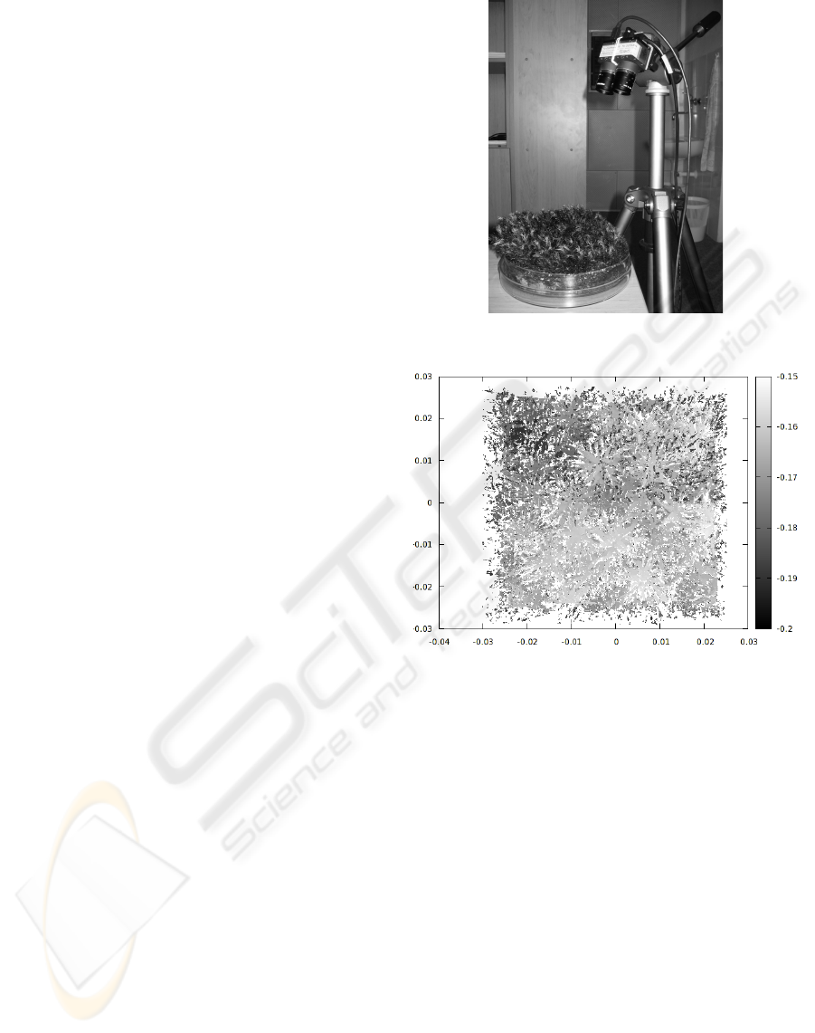
Our device is composed of hardware parts – op-

tical system consisting of two cameras and soft-

ware, analyzing acquired images. The images are ac-

quired from two IDS Imaging cameras (2240-M-GL,

monochromatic, 1280x1024 pixels, 1/2” CCD with

lenses PENTAX, f=12 mm, F1.4) ﬁrmly mounted in

a distance of 32.5 mm between them (Figure 2). Im-

ages has been taken in normal light, no auxiliary lamp

was used.

4.1 Surface Roughness

Surface roughness is a measurement of the small-

scale variations in the height of a physical surface of

bryophyte canopies.

For the statistical evaluation of every selected

bryophyte, we ﬁtted all measured z-component val-

ues that we obtained from the 3D reconstruction (2.1)

with a polynomial surface. This surface then repre-

sents the mean value of measured z-component. For

Figure 2: The pair of cameras mounted on the tripod.

Figure 3: Z-components from the reconstruction (Poly-

trichastrum formosum).

this step, we have already a full set of x-, y-, and z-

components (in meters) from the previous reconstruc-

tion process (Figure 3). Following ﬁgure shows an-

other reconstructed sample of the same species in the

original coordinates of the image (Figure 4).

In order to calculate the surface speciﬁc parame-

ters, we have to minimize the impact of subsoil seg-

mentation. We have performed a regression using the

polynomial expression above to interpolate the sub-

soil surface. Thus we have obtained the surface that

represents the average canopy level. The distances

from the reconstructed z-coordinates and the ﬁtting

surface were evaluated statistically.

Canopy structure can be characterized by the sur-

face characteristics. The most common measure of

statistical dispersion is the standard deviation, mea-

suring how widely z-values are spread in the sample.

Bryophyte canopy structure is also described by

parameter deﬁned by Rice as the square root of

twice the maximum semivariance (Rice et al., 2001).

BIOSIGNALS 2009 - International Conference on Bio-inspired Systems and Signal Processing

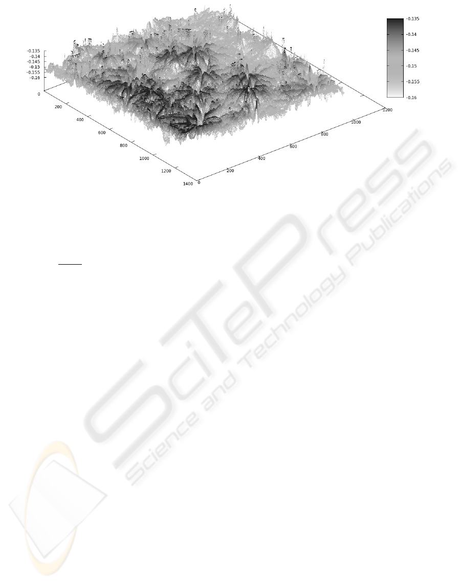
Figure 4: Results of 3D reconstruction of canopy sample (Polytrichastrum formosum).

Semivariance is described by

γ(h) =

2n(h)

n(h)

∑

i=1

(z(x

+ h) − z(x

))

, (1)

where z is a value at a particular location, h is the dis-

tance between ordered data, and n(h) is the number of

paired data at a distance of h (Bachmaier and Backes,

2008).

The real surface is so complicated that only one

parameter cannot provide a full description. For more

accurate characteristics other parameters might be

used (e.g. maximum height of the proﬁle, average

distance between the highest peak and lowest valley

in each sampling length).

5 RESULTS

When applied in a study of six bryophyte species

(Motyka et al., 2008) surface structure (Bazzania

trilobata, Dicranum scoparium, Plagiomnium undu-

latum, Polytrichastrum formosum, Polytrichum com-

mune and Sphagnum girgensohnii), both in laboratory

and in situ, mentioned approach was found to be able

to obtain data suitable for surface roughness index

calculation. Also, indices calculated in eight speci-

men per each species (four in laboratory and four in

ﬁeld measurements, total 48 specimens) were found

to signiﬁcantly distinguish the specimens in depen-

dence on species kind; one-way analysis of variance

showed high signiﬁcance (p = 0, 000108) when data

were pooled discounting whether derived from labo-

ratory or from ﬁeld measurements. Laboratory mea-

surements separate gave not that signiﬁcant outcomes

(p = 0, 0935), for there were found distinctively dif-

ferent indices of Dicranum scoparium specimens in

laboratory and in ﬁeld caused probably by disturbance

of their canopies when transferring and storage in lab-

oratory. This is supported by the fact that indepen-

dent two-sample t-test showed signiﬁcant difference

between laboratory and ﬁeld measurements outcomes

only in case of this one species (p = 0, 006976). This

approach was then found to be suitable to be utilized

even under in situ conditions which is according to

the outcomes of the mentioned study considered to

be much more convenient way to study bryophyte

canopy structure.

6 CONCLUSIONS

By comparing the results of pure stereo matching al-

gorithms (Kolmogorov and Zabih, 2001; Kanade and

Okutomi, 1994; Ogale and Aloimonos, 2005) and our

combined approach we have found out our method to

be more suitable for homochromatic surfaces. Bio-

logical samples we have been working with were typ-

ical by the presence of rather long narrow features

(leaves or branches). Heavy density of such forma-

tions in the images is more than unusual input for the

stereo matching algorithms supposing rather smooth

and continuous surfaces. Segmentation used by graph

cut based stereo matching algorithms usually lead in

creating a great many regions without match in the

second image.

Without using additional cues, described in this

paper, results of reconstructed image was poor, usu-

ally similar to noise without and further value for

bryophyte analysis. Meanwhile our reconstruction

3D RECONSTRUCTION FOR TEXTURELESS SURFACES - Surface Reconstruction for Biological Research of

Bryophyte Canopies

process produce outputs that are sufﬁcient for further

biological investigation. Both number of analyzed

specimens and number of obtained z-values for statis-

tical analysis are unprecedented and this approach is

so far the only one successfully used in ﬁeld. Further

research will be carried out in order to describe the

surface more appropriately for biological purposes.

REFERENCES

Bachmaier, M. and Backes, M. (2008). Variogram or semi-

variogram - explaining the variances in a variogram.

Precision Agriculture.

Bouguet, J.-Y. (2005). Camera calibration toolbox

for matlab. http://www.vision.caltech.edu/bouguetj/-

calib doc/index.html.

Brodie, H. J. (1951). The splash-cup dispersal mechanism

in plants. Canadian Journal of Botany, (29):224–230.

Chaudhuri, S., Rajagopalan, A., and Pentland, A. (1999).

Depth from Defocus: A Real Aperture Imaging Ap-

proach. Springer.

Coleman, Jr., E. and Jain, R. (1981). Shape from shading

for surfaces with texture and specularity. In IJCAI81,

pages 652–657.

Crum, H. (2001). Structural Diversity of Bryophytes, page

379. University of Michigan Herbarium, Ann Arbor.

Darboux, F. and Huang, C. (2003). An simultaneous-

proﬁle laser scanner to measure soil surface microto-

pography. Soil Science Society of America Journal,

(67):92–99.

Heikilla, J. (2000). Geometric camera calibration using cir-

cular control points. IEEE Transactions on Pattern

Analysis and Machine Intelligence 22, (10):1066–

1077.

Heikilla, J. and Silven, O. (1997). A four-step camera cal-

ibration procedure with implicit image correction. In

IEEE Computer Society Conference on Computer Vi-

sion and Pattern Recognition (CVPR97), pages 1106–

1112.

Horn, B. (1986). Robot Vision. MIT Press.

Horn, B. and Brooks, M. (1986). The variantional approach

to shape from shading. In Computer Vision Graphics

and Image Processing, volume 22, pages 174–208.

Howard, I. P. and Rogers, B. J. (1996). Binocular Vision

and Stereopsis, pages 212–230. Oxford Scholarship

Online.

Jarvis, R. A. (1983). A perspective on range ﬁnding tech-

niques for computer vision. In IEEE Trans. Pattern

Analysis and Machine Intelligence, volume 5, pages

122–139.

Kanade, T. and Okutomi, M. (1994). A stereo matching

algorithm with an adaptive window: Theory and ex-

periment. IEEE Transactions on Pattern Analysis and

Machine Intelligence, 16(9):920–932.

Kolmogorov, V. and Zabih, R. (2001). Computing vi-

sual correspondence with occlusions using graph cuts.

iccv, 02:508.

Liao, M., Wang, L., Yang, R., and Gong;, M. (2007). Light

fall-off stereo. Computer Vision and Pattern Recogni-

tion, pages 1–8.

Magda, S., Kriegman, D., Zickler, T., and Belhumeur, P.

(2001). Beyond lambert: reconstructing surfaces with

arbitrary brdfs. In ICCV, volume 2, pages 391–398.

Motyka, O., Krumnikl, M., Sojka, E., and Gaura, J. (2008).

New approach in bryophyte canopy analysis: 3d im-

age analysis as a suitable tool for ecological studies of

moss communities? In Environmental changes and

biological assessment IV. Scripta Fac. Rerum Natur.

Univ. Ostraviensis.

Nayar, S. K., Watanabe, M., and Noguchi, M. (1996). Real-

time focus range sensor. IEEE Transactions on Pat-

tern Analysis and Machine Intelligence, 18(12):1186–

1198.

Ogale, A. and Aloimonos, Y. (2005). Shape and the stereo

correspondence problem. International Journal of

Computer Vision, 65(3):147–162.

Ortiz, A. and Oliver, G. (2000). Shape from shading for

multiple albedo images. In ICPR, volume 1, pages

786–789.

Prados, E. and Faugeras, O. (2005). Shape from shading: a

well-posed problem? In Computer Vision and Pattern

Recognition, volume 2, pages 870–877.

Proctor, M. C. F. and Tuba, Z. (2002). Poikilohydry and

homoiohydry: antithesis or spectrum of possibilites?

New Phytologist, (156):327–349.

Rice, S. K., Collins, D., and Anderson, A. M. (2001). Func-

tional signiﬁcance of variation in bryophyte canopy

structure. American Journal of Botany, (88):1568–

1576.

Rice, S. K., Gutman, C., and Krouglicof, N. (2005). Laser

scanning reveals bryophyte canopy structure. New

Phytologist, 166(2):695–704.

Sun, J., Li, Y., Kang, S. B., and Shum, H.-Y. (2005). Sym-

metric stereo matching for occlusion handling. In

CVPR ’05: Proceedings of the 2005 IEEE Computer

Society Conference on Computer Vision and Pattern

Recognition (CVPR’05) - Volume 2, pages 399–406,

Washington, DC, USA. IEEE Computer Society.

Wedekind, J. (2002). Fokusserien-basierte rekonstruktion

von mikroobjekten. Master’s thesis, Universitat Karl-

sruhe.

Xiong, Y. and Shafer, S. (1993). Depth from focusing

and defocusing. Technical Report CMU-RI-TR-93-

07, Robotics Institute, Carnegie Mellon University,

Pittsburgh, PA.

Zhang, Z. (1999). Flexible camera calibration by viewing

a plane from unknown orientations. In International

Conference on Computer Vision (ICCV’99), Corfu,

Greece, pages 666–673.

Zhang, Z. (2000). A ﬂexible new technique for camera cal-

ibration. IEEE Transactions on Pattern Analysis and

Machine Intelligence 22, (11):1330–1334.

BIOSIGNALS 2009 - International Conference on Bio-inspired Systems and Signal Processing

100