Pearling: Stroke Segmentation with Crusted Pearl

Strings

B. Whited

, J. Rossignac

, G. Slabaugh

, T. Fang

and G. Unal

Georgia Institute of Technology, Graphics, Visualization and Usability Center

Atlanta, GA 30332, USA

Siemens Corporate Research, Intelligent Vision and Reasoning Department

Princeton, NJ 08540, USA

Abstract. We introduce a novel segmentation technique, called Pearling, for the

semi-automatic extraction of idealized models of networks of strokes (variable

width curves) in images. These networks may for example represent roads in an

aerial photograph, vessels in a medical scan, or strokes in a drawing. The operator

seeds the process by selecting representative areas of good (stroke interior) and

bad colors. Then, the operator may either provide a rough trace through a particu-

lar path in the stroke graph or simply pick a starting point (seed) on a stroke and a

direction of growth. Pearling computes in realtime the centerlines of the strokes,

the bifurcations, and the thickness function along each stroke, hence producing a

puriﬁed medial axis transform of a desired portion of the stroke graph. No prior

segmentation or thresholding is required. Simple gestures may be used to trim

or extend the selection or to add branches. The realtime performance and relia-

bility of Pearling results from a novel disk-sampling approach, which traces the

strokes by optimizing the positions and radii of a discrete series of disks (pearls)

along the stroke. A continuous model is deﬁned through subdivision. By design,

the idealized pearl string model is slightly wider than necessary to ensure that it

contains the stroke boundary. A narrower core model that ﬁts inside the stroke

is computed simultaneously. The difference between the pearl string and its core

contains the boundary of the stroke and may be used to capture, compress, visu-

alize, or analyze the raw image data along the stroke boundary.

1 Introduction

In this paper, we present Pearling, for the extraction and modeling of stroke-like struc-

tures in images. This work is motivated by the need for semi-automatic segmentation

tools, particularly in the analysis of medical images. Indeed, every year millions of

medical images are taken, many of which are used to support clinical applications in-

volving diagnosis (e.g., stenosis, aneurysm, etc.) surgical planning, anatomic modeling

and simulation, and treatment veriﬁcation. These applications either beneﬁt from, or are

required to have, a geometric model of the important structures (blood vessel, airway,

etc.) being studied. Segmentation of stroke-like structures such as blood vessels is a fun-

damental problem in medical image processing, and arises in other contexts including

industrial applications as well as aerial/satellite image analysis.

Whited B., Rossignac J., Slabaugh G., Fang T. and Unal G. (2008).

Pearling: Stroke Segmentation with Crusted Pearl Strings.

In Image Mining Theory and Applications, pages 103-112

DOI: 10.5220/0002340801030112

 SciTePress

With manual segmentation techniques, it is possible to obtain highly accurate re-

sults. However, these methods typically require an excessive amount of tedious labor to

be practical in a clinical workﬂow. While fully automatic segmentation methods can be

desirable in these applications, given the poor contrast, noise, and clutter that is com-

mon to medical images, it is often difﬁcult for fully automatic segmentation methods

to yield robust results. Furthermore, often one is interested in extracting only a sub-

set, for example a speciﬁc path through a branching network of stroke-like structures.

Therefore, there is a salient need for interactive segmentation methods that are mostly

automatic, but do accept input from the operator to guide the segmentation in a particu-

lar direction, quickly correct for errant segmentations, and add branches to an existing

segmentation result. Crucial to such a semi-automatic segmentation method is computa-

tional efﬁciency, so that the operator will not have to wait for segmentation results while

interacting with the data. Furthermore, to support further analysis or close-up visualiza-

tion it may be important to identify the portion of the image (crust) that surrounds the

stroke boundary.

1.1 Related Work

Given its clinical importance, the problem of vessel segmentation has received a fair

amount of attention in the literature. Kirbas et al. [1] present a recent survey that pro-

vide a recent survey of techniques for vessel segmentation. They conclude that there is

no single vessel segmentation approach that is robust, automatic, and fast, and that suc-

cessfully extracts the vasculature across all imaging modalities and different anatomic

regions. Following their conclusion, we step away from total automation and instead fo-

cus in interactive segmentation, providing an efﬁcient system for an operator to quickly

extract the region and branches of interest.

Other recent vessel segmentation approaches in the medical imaging literature in-

clude [2], who model vessel segments using superellipsoids, [3], who implement co-

dimension two level set ﬂows, and [4], who apply a Bayesian classiﬁer to feature vec-

tors produced using Gabor wavelets. While elegant, these techniques require signiﬁcant

computational resources. Fast methods such as [5] perform the segmentation on slices

made in a direction orthogonal to the vessel centerline or intensity maxima [6] and

then extract the vessel geometry by connecting the results. More closely related to our

work is [7], who build tunnels modeled as a union of spheres, placed through protein

molecules using a Voronoi diagram pre-computed on a segmented version of the image.

Unlike this work, our method is image-based and designed for segmentation, placing

the pearls using local pixel intensity inside each pearl.

Several authors proposed to compute skeletons through the advection of mass along

the distance ﬁeld [8] [9]. The thinning methods [10] and the methods based on distance

transform [11] for extracting a skeleton are not easily applicable to our problem of

rapidly segmenting a subset of the volume because they are global and hence slow

and require the precomputation of a distance ﬁeld. The distance ﬁeld pre-computation

may be avoided in methods that use a general scalar ﬁeld [12]. Minimal paths through

vessels have been computed using fast marching techniques [13] that backtrack along a

distance ﬁeld [14] computed with a Riemannian metric.

104104

Also related is the computation of the medial axis transform [15]. Once an image is

segmented and pixels have been identiﬁed that are in the stroke network, techniques for

selecting the center line and medial axis could be used. Pearling produces directly the

puriﬁed result that could be derived by removing automatically small branches from

the MAT and selecting a desired portion of the graph, all without requiring a prior

segmentation.

The application of this technique to tracing 3D networks of vessels has been dis-

cussed [16], but is not the same paradigm as input is more tedious and requires a differ-

ent user interaction.

1.2 Our Contribution

Pearling is a novel method for segmentation of stroke networks in images. Pearling per-

forms a segmentation and idealization simultaneously by computing an ordered series

of pearls, which are disks of possibly different radii. Starting with an initial pearl given

by the operator, as well as an initial direction, pearling iteratively computes the position

and radius of an adjacent pearl based on the image data, so that the newly placed pearl

ﬁts properly along the stroke, slightly building bulging out on both sides. The method

proceeds in this fashion, producing a string or network of strings of pearls that pro-

vide a discrete representation of the stroke geometry. Pearling is robust to ﬂuctuations

in image intensities (due to noise, etc.) as the forces acting on a pearl are integrated

over the region inside the pearl. A ﬁnal smooth contour representing the stroke net-

work is then obtained by estimating continuous functions that interpolate the discrete

series of pearls. As we will show, pearling is computationally efﬁcient and well suited

to user interactivity. This interactivity affords operator guidance of the segmentation in

a particular direction as well as operator correction of errant segmentation results.

In addition to pearls, we introduce the concepts of core and crust. The core of the

pearling model is computed by reducing the radius of each pearl while keeping its

center in place. The radius is chosen to be as large as possible, while ensuring that

a given majority of pixels inside the core pearl are good. The difference between the

“outer” pearl model and its core is the crust, which may be used to capture, compress,

archive, transmit, visualize, or analyze the original data along the stroke border. We

show in Section 3 that the crust is a narrow band around the stroke border computed

through region growing techniques.

2 Methodology

Pearling allows the operator to extract a higher level idealized parametric representation

of each stroke. This representation is called a string. As shown in Figure 1, it comprises

an ordered series of pearls (or disks), each deﬁned by the location c

of its center, by its

radius r

, and a time value t

, and possibly other attributes a

. The continuous model of

the corresponding stroke that is recovered by Pearling is deﬁned as the region W swept

by a pearl whose center c(t) and radius r(t) are both continuous and smooth functions

of the time parameter t. These functions interpolate the centers and radii of the string

of pearls for given values t

of time. For a network of strokes, multiple strings will be

deﬁned which meet at bifurcation pearls, which will be deﬁned later.

105105

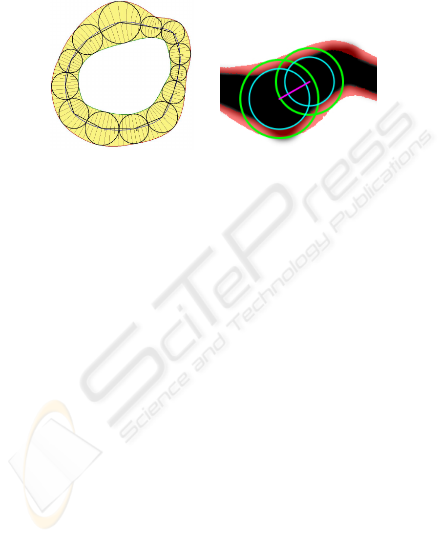
Fig. 1. Representation of Pearling, which con-

sists of an ordered series of pearls. Continu-

ous functions that interpolate the pearls are

also shown: the blue curve interpolates the

pearl centers, and the red and green curves in-

terpolate the outside and inside edges of the

pearls, respectively.

Fig. 2. Two adjacent Pearls (green) and their

cores (cyan) with their centers connected

(magenta) overlaid on top a stroke (black) and

the crust region deﬁned by the continuous set

of pearls minus their cores (red).

2.1 Estimation of Pearls

Pearling starts with an initial seed, c

, which is a point either provided by an operator or

by an algorithm. Typically, c

should be chosen to lie close to the centerline of a stroke

and possibly at the end of one of the strokes of the desired structure. Pearling then uses

an iterative process to construct an ordered series of pearls, one at a time. During that

process, at each step, the center c

and radius r

of the current pearl is chosen so as

to maximize r

subject to image data, given the constraint that the distance d

between

and the center c

i−1

of the previous pearl is bound by functions d

min

i−1

, r

) and

max

i−1

, r

). We use linear functions d

min,max

i−1

, r

) = ar

i−1

+ br

, and with

bounds d

min

i−1

, r

) = r

/2 and d

max

i−1

, r

) = r

i−1

+ r

. It is important that

be allowed to ﬂuctuate in order to capture rapid changes in thickness and allow

convergence to local minima.

Let c

i−1

be the center of the previous pearl seed, as shown in Figure 2. Let c

the center of the next pearl, and let r

be its radius. The objective is to ﬁnd the optimal

values of c

and r

that place the ith pearl in the stroke. The location of c

may be

speciﬁed in polar coordinates around c

i−1

. In order to adjust the values of r

and c

that the pearl better ﬁts snugly astride the stroke, we deﬁne two functions: f (c

, r

) and

g(c

, r

), as described below.

Center Estimation. The function f (c

, r

) returns a gradient indicating the direction

in which c

should be adjusted and the amount of the adjustment. This adjustment can

then be converted to an angle relative to c

i−1

and applied to o

. f(c

, r

) takes the form,

106106

f (c

, r

) =

2πr

x∈P

φ(x)(c

− x)



1 −

− xk



dx (1)

φ(x) =



1, if ˆp

out

(I(x)) > ˆp

(I(x))

0, otherwise

(2)

The function f (c

, r

) sums the vectors (c

− x), where x is the vector coordinate of the

the current pixel, across the entire area of pixels for pearl P

, using only those pixels

such that φ(x) = 1, i.e., pixels determined to be outside the stroke. Each of these

vectors is weighted by its distance from c

such that pixels nearer c

have a stronger

inﬂuence on the result, as reﬂected in the



1 −

−xk



component of Equation 1.

Intuitively, Equation 2 states that each point inside the ith pearl but outside the stroke

imparts a force on the pearl that pushes it away from the stroke boundary. When the

forces are balanced on all sides of the pearl, the pearl is typically centered in the vessel.

The

2πr

is a normalization factor computed by looking at the case where a pearl is cut

into two equal halves by a linear boundary separating good and bad pixels. By assuming

this ideal case, we can compute the factor by calculating the offset needed to move this

pearl half the minimum distance that would move it entirely in the good region.

Determination of whether a pixel lies inside the stroke or outside the stroke is

necessary when computing f (c

, r

), and is achieved using non-parametric density es-

timation. Before running the algorithm, the operator selects two regions; one inside

the stroke and one outside. For a given region, we estimate the density by applying a

smoothing kernel K to the pixels in the region’s histogram, i.e.,

ˆp =

i=1



− m



, (3)

where I

is the intensity of the ith pixel in the region, m is the mean of intensities of

the n pixels in the region, and h is the bandwidth of the estimator. We use a Gaussian

kernel, K(u) =

√

2π

−

. Performing this estimation on two operator-supplied re-

gions results in two densities, ˆp

(I) and ˆp

out

(I). During segmentation, an intensity I

is classiﬁed as outside if ˆp

out

(I) > ˆp

(I); otherwise it is classiﬁed as inside.

Radius Estimation. r

is adjusted to better ﬁt the stroke using the function g(c

, r

as shown in Equation 4. For robustness, pearls are designed to have a percentage p of

their pixels inside the tube and the rest outside the tube, as indicated in Figure 2. In our

implementation, g(c

, r

) is positive when less than p percent of the pearl’s pixels ﬁt in

the tube and negative more than 1 − p of the pixels lie outside of the tube. The portion

of the enlarged pearl that lies outside of the tube is typically computed by sampling the

pearl’s interior, however, alternatively one can sample the pearl’s boundary. The result

of g(c

, r

) is then used to scale r

to better ﬁt in the tube. g(c

, r

) takes the form,

g(c

, r

) = p −

x∈P

(1 − φ(x)) dx

x∈P

(4)

107107

Interleaving the Estimation and Convergence. We interleave the estimation of c

and

for the ith pearl P

. For a given position c

and radius r

, one can update both param-

eters independently using the results given by f (r

, c

) and g(r

, c

). In both cases, the

quality of the ﬁt is measured and the desired adjustment is computed and returned.

The adjustments of c

and r

are done through several iterations while enforcing

the constraint on d

until the adjustment values returned by f (c

, r

) and g(c

, r

) fall

below a given threshold. The process then freezes the current pearl and starts ﬁtting the

next one. The growth of a stroke stops when the radius of the next pearl falls outside

of a prescribed range, or when another application-dependent criterion is met, such as

the detection of an operator-supplied endpoint. The result of this Pearling process is a

series of location-radius pairs (c

, r

), which we call the control pearls.

2.2 Direction Estimation and Bifurcations

Often in the applications targeted, images contain sharp turns and bifurcations where a

stroke will branch into multiple strokes and may even contain loops. We have extended

the above process to support these options.

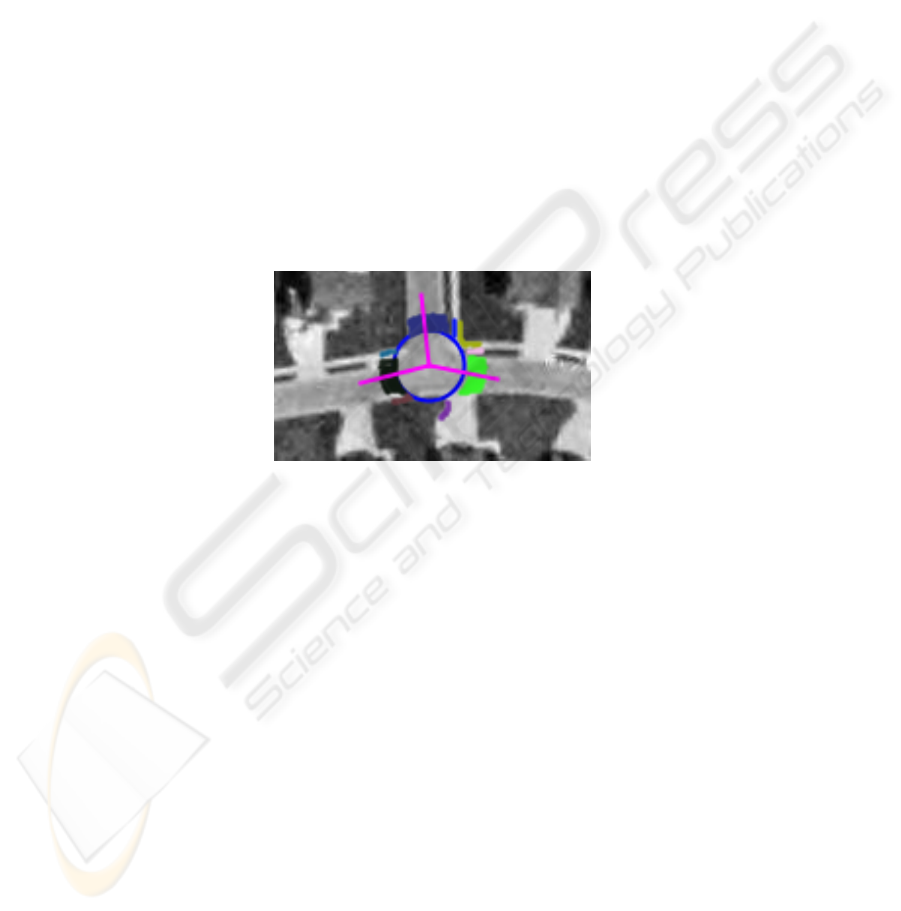
Fig. 3. A pearl shown at a stroke bifurcation along with its set of good pixels in the region

bounded by r

and kr

. Each connected component C

is uniquely colored. Vectors D

(ma-

genta) are shown for the connected components which contain a number of pixels greater than

the set threshold.

Once a pearl P

has converged to ﬁt on a stroke, an analysis of the region around P

is done in order to decide where to initially position P

i+1

, taking into account that

there could be more than one P

i+1

or none. This analysis is done on the pixels in a

circular band around P

with an outer radius kr

where k is some constant . For our

results, a value of k = 1.35 is used. Each pixel x in this band is then classiﬁed using

Equation 2. The result gives a classiﬁcation with N > 0 connected components of

good pixels. At minimum, there should be a connected component identifying the path

from the previous pearl, P

i−1

. If N = 1, then the only possible direction is backwards

and pearling stops growing the current branch because its end has been found. If N >

1, then the starting position(s) for any subsequent pearl(s) can be chosen using the

remaining connected components. For each connected component C

, an average point

is calculated which deﬁnes a direction vector D

from the pearl center c

. Subsequent

pearls are then initialized to the points on the boundary points of P

which intersect

108108

each D

. This extension allows pearling to accommodate sharp turns and bifurcations

in the stroke structure.

A loop in the pearling network can also exist. A simple intersection check between

the current pearl and all previous pearls will reveal if such a loop has occurred. In this

case, the current pearl is linked to the intersected pearl and its string is ended. The

intersected pearl could then become a bifurcation pearl, if it already has more than one

adjacent pearl, or it could be the end of another stroke still in in the growing phase. If

the latter is the case, and two growing strokes collide, they are both ended and become

part of the same stroke.

2.3 Building a Continuous Model

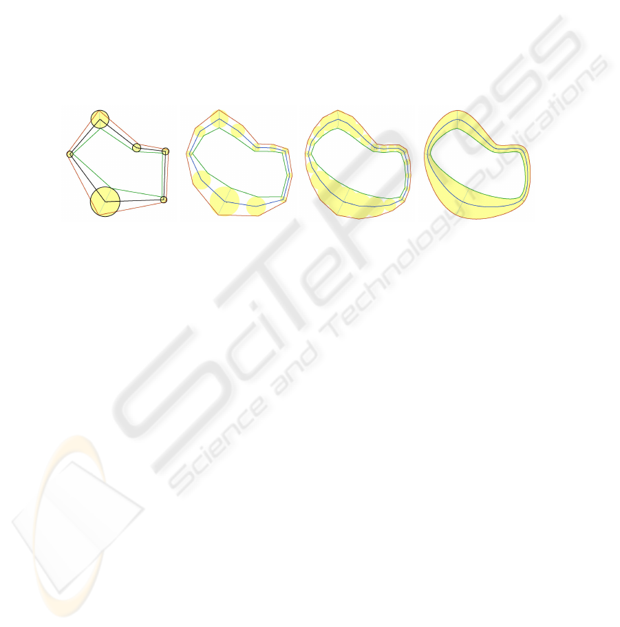
Fig. 4. Subdivision for estimating the continuous canal surface that interpolates the pearls.

A continuous model W of each stroke is obtained by computing continuous functions

c(t) and r(t) that interpolate the discrete set of end, branching and contour pearls. We

model W as the union of an inﬁnite set of disks [17], which is and may be expressed in

parametric form as W = Disk(c(t), r(t)) for t ∈ [0, 1]. If we assume that the pearls are

more or less uniformly spaced along the stroke, we can deﬁne the string as the limit of a

four-point subdivision process, which, at each iteration, introduces a new pearl between

each pair of consecutive pearls as shown in Fig 4.

3 Results

We now present segmentation results using Pearling. We begin with the segmentation of

a satellite image of a river. The original image with the initial inputs is shown in Figure 5

(left). As described, the initial inputs include regions of good and bad pixels (shown in

green and red) and an initial point and direction (shown in orange). The algorithm then

proceeds, successively adding pearls until no more can be added, the result of which is

shown in Figure 5 (center). From the collection of discrete pearls and their cores, we

can then extract the continuous model of the crust, as seen red in Figure 5 (right). The

yellow region in the ﬁgure is the result of a simple region-growing segmentation using

the same good and bad regions and starting point as pearling. A zoomed-in section

shows almost all boundary pixels are contained within the pearling crust.

109109

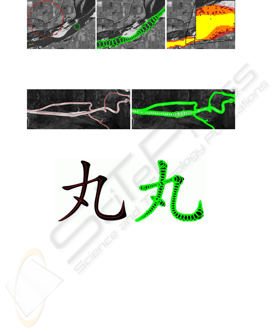
Fig. 5. An unedited grayscale image obtained from satellite imagery of a river shown with the

initial inputs(left), the resulting pearling segmentation, computed in 33ms(center), and the crust

(red) overlaid atop a simple region-grown segmentation (yellow), showing that the majority of

boundary details are contained within the crust.

Fig. 6. An MR angiographic image with centerlines(left) and discrete pearls (right) computed by

pearling in 27ms on an image with size 436x168.

Fig. 7. A Chinese character with centerlines(left) and discrete pearls (right) computed by pearling

in 37ms on an image with size 236x201.

Figures 6 and 7, present more segmentation results, of an MR angiographic image, and

a variable width Chinese character. For each ﬁgure, we show the original image with the

pearling-computed centerlines (left) and the pearl disks (right). Note that all examples

completed in tens of milliseconds.

3.1 User Interactivity

As Pearling is computationally efﬁcient, it affords the user interaction with data without

delays. In Figure 8 (left) we show an example where an operator can select a string by

simply moving the mouse over any pearl in the string. Once selected, the branch can

110110

Fig. 8. An initial incomplete pearling, with one string selected (yellow) by the operator (left). The

result of the deleting the selected string and also the initial input for a new string (orange) by the

operator (center), and the result (right).

then be deleted with the press of a key, as shown in Figure 8 (center). The operator can

also add strings to an incomplete segmentation by simply selecting a pearl and drawing

a new direction vector from it, as shown in orange in Figure 8 (center). The result of the

new string being grown is shown in Figure 8 (right).

For more control, the operator may provide a rough trace of the centerline of a

desired stroke. As the operator is manually tracing, pearls are placed at samples along

the curve and converge in real-time thus forming the stroke as the operator is tracing

it with a stylus. In this mode, the operator uses a stylus to quickly trace a rough curve

through the desired stroke structure and then as desired, adds branches. A preset mode

or the stylus speed when the stylus is released indicate how far past the release point will

pearling grow the stroke structure. As the operator is still tracing the curves, pearling

computes the idealized strokes (centerline and radius) and displays them. Each new

trace either adds or removes a branch.

4 Conclusions

In this paper we presented Pearling, a new method for semi-automatic segmentation

and geometric modeling of stroke-like structures. Pearling performs a segmentation by

computing an ordered series of pearls that discretely model the stroke structure geom-

etry. Smoothing is used to deﬁne a continuous model. The computational efﬁciency of

Pearling affords efﬁcient user interaction with the segmentation, allowing the opera-

tor to correct for errant segmentation results or guide the segmentation in a particular

direction through the data.

Sometimes the idealized pearling result doesn’t contain enough information to per-

form a more precise analysis, so we presented the concept of a crust around the border

region. Important image information, such as the inner wall of an artery, is identiﬁed in

the crust region and can be used to support a more detailed analysis.

While more comprehensive validation of the algorithm is required, from our ex-

perimental results we conclude that Pearling results in highly efﬁcient segmentation of

strokes, and holds much promise for semi-automatic image segmentation.

111111

References

1. C. Kirbas, F. Quek, A Review of Vessel Extraction Techniques and Algorithms, ACM Com-

puting Surveys 36 (2) (2004) 81–121.

2. J. A. Tyrrell, E. di Tomaso, D. Fuja, R. Tong, K. Kozak, R. Jain, B. Roysam, Robust 3-D

Modeling of Vasculature Imagery Using Superellipsoids, IEEE Trans. on Medical Imaging

26 (2) (2007) 223–237.

3. L. M. Lorigo, O. D. Faugeras, W. E. L. Grimson, R. Keriven, R. Kikinis, A. Nabavi, C.-

F. Westin, CURVES: Curve Evolution for Vessel Segmentation, Medical Image Analysis 5

(2001) 195–206.

4. J. Soares, J. Leandro, R. Cesar, H. Jelinek, M. Cree, Retinal Vessel Segmentation Using the

2-D Gabor Wavelet and Supervised Classiﬁcation, IEEE Trans. on Med. Img. 25 (9) (2006)

1214–1222.

5. O. Wink, W. Niessen, M. A. Viergever, Fast delineation and visualization of vessels in 3-d

angiographic images, IEEE Trans. on Medical Imaging 19 (4) (2000) 337–346.

6. A. Szymczak, A. Tannenbaum, K. Mischaikow, Coronary vessel cores from 3D imagery:

a topological approach, in: Medical Imaging 2005: Image Processing. Proceedings of the

SPIE, Vol. 5747, 2005, pp. 505–513.

7. P. Medek, P. Benes, J. Sochor, Computation of tunnels in protein molecules using Delaunay

triangulation, in: Journal of WSCG, 2007, p. 8.

8. L. Costa, R. Cesar, Shape Analysis and Classiﬁcation, CRC Press, 2001.

9. A. Telea, J. J. van Wijk, An augmented fast marching method for computing skeletons and

centerlines, in: Symposium on Data Visualisation, 2002, pp. 251–259.

10. C. Pudney, Distance-ordered homotopic thinning: A skeletonization algoritm for 3D digital

images, IEEE. Trans. on Biomedical Engineering 72 (3) (1998) 404–413.

11. M. Van Dortmont, H. van de Wetering, A. Telea, Skeletonization and distance transforms of

3d volumes using graphics hardware, in: DGCI, 2006, pp. 617–629.

12. N. Cornea, D. Silver, X. Yuan, R. Balasubramanian, Computing hierarchical curve-skeletons

of 3d objects, The Visual Computer 21 (11) (2005) 945–955.

13. H. Li, A. Yezzi, Vessels as 4D Curves: Global Minimal 4D Paths to 3D Tubular Structure

Extraction, in: Workshop on Mathematical Methods in Biomedical Image Analysis, 2006.

14. L. D. Cohen, R. Kimmel, Global minimum for active contours models: A minimal path

approach, IJCV 24 (1) (1997) 57–78.

15. H. Blum, A Transformation for Extracting New Descriptors of Shape, in: W. Wathen-Dunn

(Ed.), Models for the Perception of Speech and Visual Form, MIT Press, Cambridge, 1967,

pp. 362–380.

16. B. Whited, J. Rossignac, G. Slabaugh, T. Fang, G. Unal, Pearling: 3d interactive extraction

of tubular structures from volumetric images, in: MICCAI Workshop: Interaction in Medical

Image Analysis and Visualization, 2007.

17. G. Monge, Applications de l’analyse

a la g

eom

etrie, 5th Edition, Bachelier, Paris, 1894.

112112