DIAGNOSIS OF DISCRETE EVENT SYSTEMS WITH
PETRI NETS AND CODING THEORY
Dimitri Lefebvre
GREAH – University Le Havre, France
Keywords: Diagnosis, discrete event systems, Petri net models, events estimation.
Abstract: Event sequences estimation is an important issue for fault diagnosis of DES, so far as fault events cannot be
directly measured. This work is about event sequences estimation with Petri net models. Events are assumed
to be represented with transitions and firing sequences are estimated from measurements of the marking
variation. Estimation with and without measurement errors are discussed in n – dimensional vector space
over alphabet Z
3
= {-1, 0, 1}. Sufficient conditions and estimation algorithms are provided. Performance is
evaluated and the efficiency of the approach is illustrated on two examples from manufacturing engineering.
1 INTRODUCTION
Modern technological processes include complex
and large-scale systems, where faults in a single
component have major effects on the availability and
performances of the system as a whole. For example
manufacturing systems consists of many different
machines, robots and transportation tools all of
which have to correctly satisfy their purpose in order
to ensure and fulfil global objectives. In this context,
a failure is any event that changes the behaviour of
the system such that it does no longer satisfy its
purpose (Rausand et al., 2004). Faults can be due to
internal causes as to external ones, and are often
classified into three subclasses: plant faults that
change the dynamical input – output properties of
the system, sensor faults that results in substantial
errors during sensors reading, and actuator faults
when the influence of the controller to the plant is
disturbed. In order to limit the effects of the faults on
the system, diagnosis is used to detect and isolate the
failures. Diagnosis includes distinct stages: the fault
detection decides whether or not a failure event has
occurred; the fault isolation find the component that
is faulty; the fault identification identifies the fault
and estimates also its magnitude. Model-based and
data-based methods have been investigated for
diagnosis (Blanke et al., 2003).
The motivations for the diagnosis of discrete
event system (DES) are obvious as long as DES
occur naturally in the engineering practice. Many
actuators like switches, valves and so on, only jump
between discrete states. Binary signals are mainly
used with numerical systems and logical values
“true” and “false” are often used as input and output
signals. Alarm sensors that indicate that a physical
quantity exceeds a prescribed bound are typical
systems with only two logical states. Moreover, in
several systems also the internal state is discrete
valued. As an example, robot encoders are discrete
valued even if the number of discrete state is large
enough to produce smooth trajectories. At last, one
must keep in mind that a given dynamical system
can always be considered as a DES system or as a
continuous variable system according to the purpose
of the investigation. As long as supervision
problems are considered, a rather broad view on the
system behaviour can be adopted that is based on
discrete signals. On the contrary, if signals have to
remain in a narrow tolerance band, the following
approaches do no longer fit and one has to adopt a
continuous point of view (Blanke et al., 2003).
The behaviour of DES is described by sequences
of input and output events. In contrast to the
continuous systems only abrupt changes of the
signal values are considered with DES. In that case,
the problem has been originally investigated with
observation methods for automata developed in
connection with the supervisory control theory
(Ramadge et al., 1987). Concerning model-based
methods automata (Sampath et al., 1995) or Petri
nets (Ushio et al. 1998) models can be used. This
article focus on diagnosis of DES modelled with
Petri nets (PN) where failures are represented with
some particular transitions. The problem is to detect
and isolate the firing of the failure transitions in a
15
Lefebvre D. (2008).
DIAGNOSIS OF DISCRETE EVENT SYSTEMS WITH PETRI NETS AND CODING THEORY.
In Proceedings of the Fifth International Conference on Informatics in Control, Automation and Robotics - RA, pages 15-22
DOI: 10.5220/0001481700150022
Copyright
c
 SciTePress

given firing sequence. The firings of the failure
transitions are assumed to be unobservable and must
be estimated according to complete or partial
marking measurements that are eventually disturbed
by measurement errors. As a consequence a method
based on coding theory is proved to be suitable for
sensor faults diagnosis. The article is divided into six
sections. Section two is about Petri nets states.
Section three states the diagnosis problem for DES
and is about the usual state space methods for PN.
Section four details the event estimation with coding
theory that can be combined with state space
approach. Both methods are presented in a
framework in the conclusion.
2 ORDINARY PETRI NETS
An ordinary PN with n places and q transitions is
defined as < P, T, Pre, Post > where P = {P
i
} is a
non-empty finite set of n places, T = {T
j
} is a non-
empty finite set of q transitions, such that P ∩ T =
∅. Pre: P × T → {0, 1} is the pre-incidence
application and W
PR
= ( w
PR
ij
) ∈ {0, 1}
n
×
q
with
w
PR
ij
= Pre (P
i
, T
j
) is the pre-incidence matrix. Post:
P × T → {0, 1} is the post-incidence application and
W
PO
= ( w
PO
ij
) ∈ {0, 1}
n
×
q
with w
PO
ij
= Post (P
i
, T
j
)
is the post-incidence matrix. The PN incidence
matrix W is defined as W = W
PO
– W
PR
∈ Z
3
n x q
with Z
3
∈ {-1, 0, 1} and w
i
stands for the i
th
column
of W (Askin et al., 1993; Cassandras et al., 1999;
David et al., 1992). M = (m
i
) ∈ (Z
+
)
n
is defined as
the marking vector and M
I
∈ (Z
+
)
n
as the initial
marking vector, with Z
+
the set of non negative
integer numbers. A firing sequence σ = T
i
.T
j
… T
k
is
defined as an ordered series of transitions that are
successively fired from marking M to marking M’
(i.e. M [σ > M’) such that equation (1) is satisfied:
}} }
σ→→→→L
j
k
i
T
T
T
12
:M M M M'
(1)
A sequence σ can be represented by its
characteristic vector (i.e. Parikh vector) X = (x
j
) ∈
(Z
+
)
q
where x
j
stands for the number of times T
j
has
occurred in sequence σ (David et al., 1992).
Marking M’ resulting from marking M with the
execution of sequence σ is given by (2) where X is
the characteristic vector for sequence σ:
ΔM = M’ - M = W.X
(2)
The reachability graph R(PN, M
I
) is the set of
markings M such that a firing sequence σ exists
from M
I
to M. A sequence σ is said to be executable
for marking M
I
if there exists a couple of markings
(M, M’) ∈ R(PN, M
I
) such that M [σ > M’.
3 DIAGNOSABILITY AND
DIAGNOSER DESIGN FOR DES
3.1 Problem Statement
In the context of diagnosis, it is commonly assumed
that no inspection of the process is possible. As a
consequence the diagnosis is only based on available
measurement data. Basically, the diagnosis problem
for a dynamical system with input u, output y and
subject to some faults f, is to detect and isolate the
faults from a given sequence of input – output
couples (U, Y) with:
U = (u(0), u(1),…,u(k))
Y = (y(0), y(1),…,y(k))
(3)
where k stands for time t = k.Δt, and Δt represents
the sampling period of sensors. The main issues are
(1) to decide the diagnosability of the faults; (2) to
detect, isolate and identify the faults that are
diagnosable. In case of model - based diagnosis, the
input – output couples (U, Y ) are usualy compared
with the behaviour of a reference model. Fault
indicators like residuals are worked out from this
comparison. It is often convenient to separe actuator,
system and sensor faults.
As long as DES are considered the inputs and
faults are usualy considered as events and the
outputs are related to the states of the DES. A
reference model (automata, finite state machines,
Petri nets, and so on) can be used for diagnosis
purpose and sequences of estimated outputs obtained
thanks to the model are compared with the measured
outputs of the system. Indicators of the faults result
from this comparison. According to the traces
generated by the system, faults are :
(1) strongly diagnosable if they result in immediate
abnormal behaviours (no intermediate event is
required for diagnosis);
(2) weakly diagnosable if they result in abnormal
behaviours after a finite number of intermediate
events;
(3) non diagnosable if no abnormal behaviour
occurs whatever the future evolution of the
system.
Let us notice that the notion of strong or weak
diagnosability for DES is related to the question of
persistent excitation in temporal systems.
ICINCO 2008 - International Conference on Informatics in Control, Automation and Robotics
16

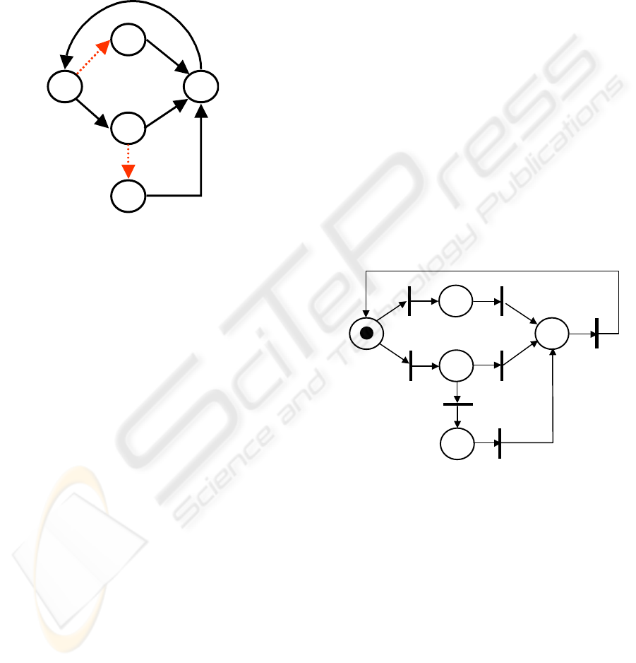
The figure 1 is an example of diagnosis with finite
state machine. The system has 5 states {A, B, C, D,
E}, 4 outputs {1, 2, 3, 4}, 5 inputs {a, b, c, f
1
, f
2
} (3
normal events {a, b ,c} and 2 fault events {f
1
, f
2
}).
The reference model (full lines only) and the system
(full and dashed lines) evolve according to the figure
1. Diagnosability analysis and diagnosers design
result from the simulation with automata in figure 1.
Figure 1: Example of diagnosis with finite state machine.
If the state of the system is measured, then the
faults f
1
and f
2
are both strongly diagnosable as long
as the fault events lead to an immediate difference
between system state (S) and estimated one (S
est
)
(table 1, grey cells). If only the output is measured
then the fault f
2
is strongly diagnosable but the fault
f
1
is weakly diagnosable in the sense that
intermediate event “b” must occur so that the system
output (O) and estimated output (O
est
) become
different. If state “E” results in output “1” instead of
“4” then fault f
2
is non diagnosable.
3.2 Diagnosis with Petri Nets
The previous approach can be applied to Petri net
models with finite reachability graph to prove the
diagnosability of the faults and to design diagnosers
based on Petri net models. The basis idea is to
investigate the indeterminate cycles in partial
expansion of the reachability graph (Ushio et al.,
1998). The considered PN are live (i.e. for any T
j
∈
T, and for all M ∈ R(PN, M
I
) there exists a sequence
σ executable from M that includes transition T
j
) and
safe (i.e. for all M ∈ R(PN, M
I
), M ∈ {0, 1}
n
). Some
places are assumed to be observable and other not,
and transitions, that are associated with events, are
usually assumed to be unobservable. A cycle is
called “determined” if it contains at least one
observable state that results with no ambiguity from
a normal firing sequence, or from a firing sequence
with a fault. The fault is diagnosable if and only if
there is no indeterminate cycle in partial expansion
of the reachability graph that correspond to the
observable part of the system. For a diagnosable
fault, the detection and isolation can be obtained
according to the finite state machine that corresponds
to partial expansion of the reachability graph. Let us
notice that the method is different from the dignosis
with finite state machines in the sense that
knowledge of inputs is not required and that
definition of outputs is restricted to marking
projection.
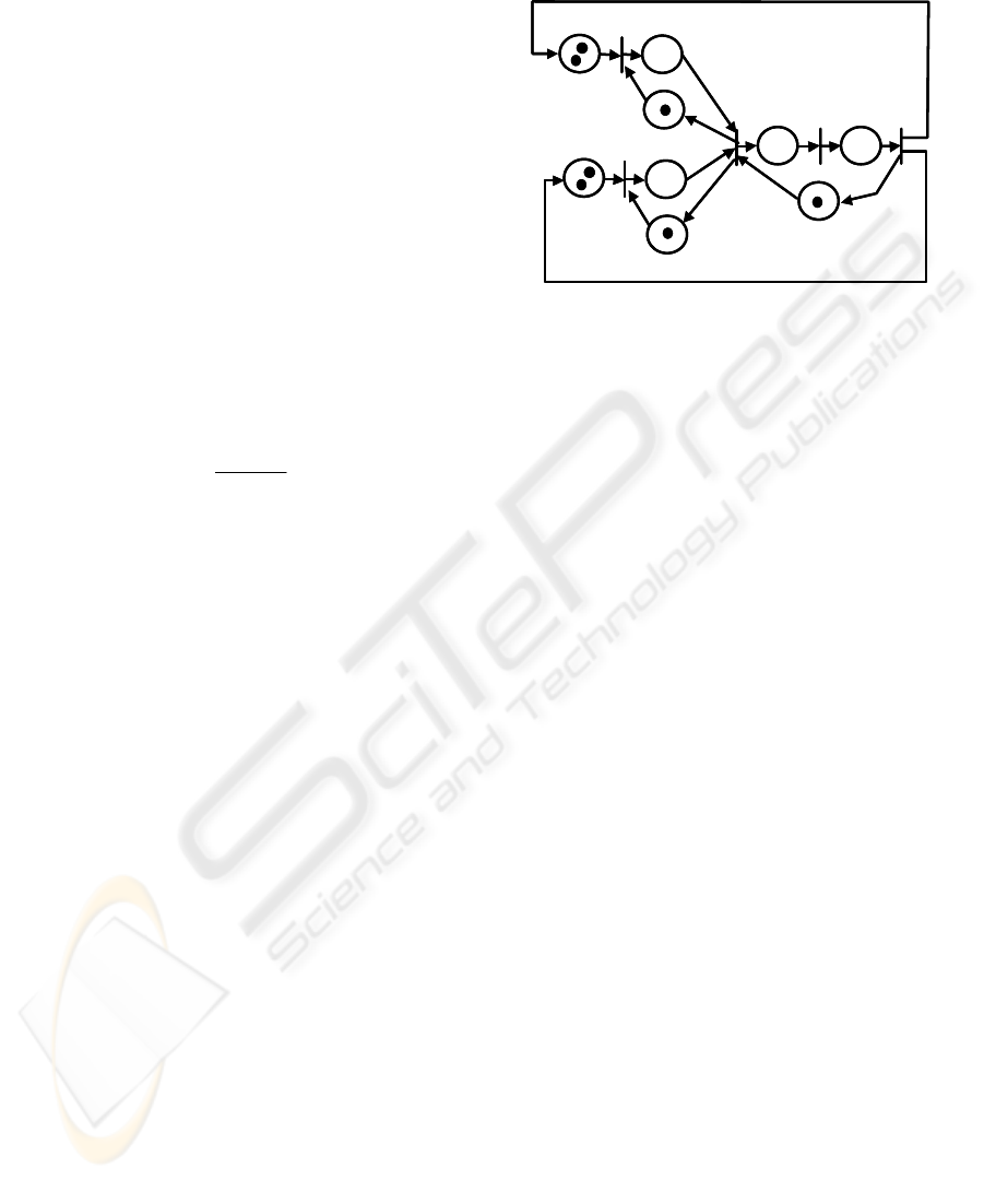
Let consider the system PN1 in figure 2 as an
example
. The reachability graph of PN1 is the finite
state machine of figure 1.
If the set of observable
places is given by P
O1
= {P
1
, P
4
, P
5
}, the observable
part of the labelled reachability graph R(PN1, {T
1
},
(1, 0, 0, 0, 0)
T
, P
O1
) is worked out as in figure 3a.
This diagnoser has an indetermined cycle so the
system is not diagnosable (figure 3a, left cycle). If
P
O2
= {P
1
, P
3
}, the observable part of the labelled
reachability graph R(PN1, {T
1
}, (1, 0, 0, 0, 0)
T
, P
O2
)
is worked out as in figure 3b. This diagnoser has no
indetermined cycle so the system is diagnosable.
Figure 2: Example PN1 of Petri net.
Let us mention that other approaches have been
developped for diagnosis based on event
detectability (Ramirez – Trevino et al., 2007) and
structural properties (Lefebvre et al., 2007). All
above mentioned approaches require complete or
partial measurements of the marking vector. Thus,
they are sensitive to measurement errors. As a
consequence, it is important to detect and eventually
correct the errors that disturb the measurements of
marking variation in order to obtain an exact
estimation of the occurrence of events. The next
section concerns events estimation and can be
introduced as a diagnosis method for sensor faults.
A
/
1
B
/
1
C/
2
E
/
4
D/3
b
a
b
b f
1
f
2
c
P
1
P
2
P
3
P
4
P
5
T
2
(a)
T
1
(f
1
)
T
3
(a)
T
4
(b)
T
5
(f
2
)
T
6
(b)
T
7
(c)
DIAGNOSIS OF DISCRETE EVENT SYSTEMS WITH PETRI NETS AND CODING THEORY
17

Table 1: Example of input sequence (I), state sequence (S), output sequence (O), estimated state sequence (S
est
) and
estimated output sequence (O
est
) for the final state machine in figure 1
I a b c a f
2
b C f
1
b c a b …
S C E A C D E A B E A C E …
O 2 4 1 2 3 4 1 1 4 1 2 4 …
S
est
C E A C C E A A A A C E …
O
est
2 4 1 2 2 4 1 1 1 1 2 4 …
Figure 3 : Two partial expansions of the reachability graph
for PN1 a) R(PN1, {T
1
}, (1, 0, 0, 0, 0)
T
, P
O1
) ; b) R(PN1,
{T
1
}, (1, 0, 0, 0, 0)
T
, P
O2
).
4 SENSOR FAULTS DIAGNOSIS
BASED ON CODING THEORY
Event sequences estimation is an important issue for
fault diagnosis of DES, so far as fault events cannot
be directly measured. This section is about event
sequences estimation with PN models. Events are
assumed to be represented with transitions and firing
sequences are estimated from measurements of the
marking variation. Estimation with and without
measurement errors can be discussed in n –
dimensional vector space over alphabet Z
3
= {-1, 0,
1} (Lefebvre, 2008). The basis idea to correct
measurement errors by projecting measurements in
orthogonal subspace of Vect(W) where Vect(W)
stands for the subspace generated by the columns of
W. This method is inspired from linear coding theory
(Van Lint, 1999) and extends the results presented
for continuous PN in (Lefebvre et al., 2001).
Our contribution can be compared to another
method that incorporates redundancy into Petri nets
to detect and identify faults (Li et al., 2004; Wu et
al., 2002, 2005) and uses algebraic decoding
techniques as the Berlekamp – Massey decoding
(Berlekamp, 1984). The marking of the original PN
is embedded into a redundant one and the diagnosis
of faults is performed by mean of linear parity
checks. In comparison with the method developed in
(Wu et al., 2005), our approach does not require
additive places, but is less efficient for faults
correction.
Let us assume that measurement
ˆ
ΔM
of marking
variation ΔM ∈ (Z
3
)
n
may be affected by additive
error vector E ∈ (Z
3
)
n
:
Δ
=Δ +
ˆ
MME
where “+”
stand for the sum endowed over Z
3
. Error vector will
be characterized according to the Hamming distance
d(W) of the considered PN that is defined with the
Hamming distance of the columns of incidence
matrix :
=≠
ij 0i
d(W) min{min{d(w ,w ),i
j
},min{d (w )}}
(4)
where d(w
i
, w
j
) stands for the Hamming distance
between columns w
i
and w
j
of matrix W and d
0
(w
i
) =
d(w
i
, 0) stands for the weight of vector w
i
.
It is assumed that error vector E verifies the
following conditions:
a) Pr(d
0
(E) = 0) > Pr(d
0
(E) = 1) > ... > Pr(d
0
(E) = n)
where Pr(d
0
(E) = i) is the probability that weight
of E equals i;
b) An error in position i does not influence other
positions;
c) A symbol in error can be each of the remaining
symbols with equal probability.
(
10000, N
)
(00010, N)
(
00001, N
)
(10000, F)
(
10000
,
N
)
(00001, F)
(
00001
,
N
)
(01000, F)
(
00100
,
N
)
(
10000, N
)
(01000, F)
(
00001
,
F
)
(00010, N)
(
00001
,
N
)
(00100, N)
(10000, F)
(00010, F)
(
00001
,
F
)
(00100, F)
a)
b)
ICINCO 2008 - International Conference on Informatics in Control, Automation and Robotics
18

A short estimation algorithm easy to use and to
implement when state measurement is complete (i.e.
all entries of
ˆ
ΔM
are measured), and error free (i.e.
measurement equals actual marking variation ΔM),
is based on the comparison of measurement with
respect to columns of W and zero vector (this
corresponds to the condition of event-detectability in
case that all places are observable). When this
measurement equals a single column of W, the
algorithm decides that the corresponding transition
fired. When it equals the zero vector, the algorithm
decides that no transition fired.
When measurement is perturbed by non zero error
E, two problems must be mentioned :
a) A miss estimation may occur when
ˆ
ΔM
is non
zero and different from any columns of W. The
estimation algorithm is not able to decide if a
transition fired or not and which transition fired.
As consequence the algorithm does not give any
decision.
b) A wrong estimation may occur when
ˆ
ΔM
does
not equal actual marking variation ΔM but
equals zero vector or another column of W. The
estimation algorithm decides if a transition fired
or not and which transition fired, but the decision
is wrong due to the measurement error.
To overcome these difficulties and to improve
estimation, diagnosis can be reformulated as a linear
problem in ((Z
3
)
n
, +, *), with the Smith
transformation of W, where “+” and “*” stand for
the sum and product endowed over Z
3
. The Smith
transformation results from elementary operations
(i.e. row or column permutations, linear
combinations and external products), summed up in
matrices P ∈ (Z
3
)
n x n
and Q ∈ (Z
3
)
q x q
such that:
⎛⎞
=
⎜⎟
⎝⎠
r
I0
P*W*Q
00
(5)
I
r
is the identity matrix of dimension r x r, and r is
the rank of matrix W. The Smith transformation
leads to reduced incidence matrix W' :
W' = (I
r
0) * Q
-1
= (I
r
0) * P *W
= F * W ∈ (Z
3
)
r x q
(6)
Necessary and sufficient conditions for firing
sequences estimation can be stated when
measurement is error free and basic assumption in
section 2.b is satisfied : columns of incidence matrix
W' defined by equation (6) are distinct and non zero
(Lefebvre, 2008). In case of measurement errors that
satisfy assumptions a to c, sufficient conditions
inspired from coding theory can be stated. These
conditions are based on Hamming distance, cosets
investigation, parity check matrices, and syndromes
(Van Lint, 1999). Cosets characterise the structure of
(Z
3
)
n
according to the sum and product over Z
3
(the
coset C(u) of u is defined as C(u) = {x ∈ (Z
3
)
n
such
that x = u + y with y ∈ Vect(W)}, for any vector u ∈
(Z
3
)
n
). Parity check matrices are introduced to work
out syndromes that can be considered as the
signatures of the faults in (Z
3
)
n
. Two conditions for
firing sequences estimation are proposed (Lefebvre,
2008):
a) Columns of incidence matrix W are distinct, non
zero and errors E that disturb satisfy d
0
(E) ≤
(d(W) – 1) / 2 (i.e. the number of disturbed
entries of measurement is no larger than (d(W) –
1) / 2).
b) Columns of reduced incidence matrix W' are
distinct and non zero, and considered errors E
belong to distinct cosets different from C(0).
Moreover, the use of the Smith transformation of
incidence matrix is also helpful to define the parity
check matrix H
T
= (0 I
n-r
) * P ∈ (Z
3
)
(n-r) x n
, and to
work out the syndrome of marking variation
measurements S(
ˆ
ΔM
) = H
T
*
ˆ
ΔM
and to compare
it with the syndrome of errors S(E) = H
T
* E. As a
consequence the method leads to a less complex and
more efficient diagnosis algorithm (algorithm b) in
comparison with usual method based on Hamming
distance (algorithm a) (Lefebvre, 2008).
Algorithm a
1. For each time k, measure
ˆ
M
(k) the current state
of DES
2. Compute
ˆ
ΔM
(k) =
ˆ
M
(k) –
ˆ
M
(k-1)
3. Compute weight d
0
(
ˆ
ΔM
(k)). If d
0
(
ˆ
ΔM
(k)) ≤
(d(W) - 1) / 2, then no event occurs between two
consecutive state measurements. Go to step 6.
4. Compute Hamming distance d(
ˆ
ΔM
(k), w
j
) for
each column w
j
of W. If d(
ˆ
ΔM
(k), w
j
) ≤ (d(W) -
1) / 2 then T
j
fired. Go to step 6.
5. If for all j = 1,...,q, d(
ˆ
ΔM
(k), w
j
) > (d(W) - 1) / 2
then measurement is too much disturbed by
errors (i.e. d
0
(E) > (d(W) – 1) / 2) and no
decision is provided (i.e. a miss estimation
occurs).
6. Wait until time k + 1. Go to step 1.
DIAGNOSIS OF DISCRETE EVENT SYSTEMS WITH PETRI NETS AND CODING THEORY
19

Algorithm b
1. For each time k, measure
ˆ
M
(k) the current state
of DES
2. Compute
ˆ
ΔM
(k) =
ˆ
M
(k) –
ˆ
M
(k-1)
3. Compute H
T
*
ˆ
ΔM
(k). If H
T
*
ˆ
ΔM
(k) = 0 then
measurement is not disturbed by errors:
Δ=Δ
ˆ
M(k) M(k) . Go to step 5.
4. If syndrome H
T
*
ˆ
ΔM
(k)≠0, compute coset leader
E(k) and
Δ=Δ−
ˆ
M(k) M(k) E(k). Go to step 5.
5. Compute ΔM'(k) = F * ΔM(k).
6. If ΔM'(k) = 0 then no event occurs between 2
consecutive state measurements. Go to step 8.
7. If ΔM'(k) = w'
j
then T
j
fired. Go to step 8.
8. Wait until time k + 1. Go to step 1.
The correction capacity (i.e. number of error
vectors that are corrected) of algorithm a is given by
equation (7):
−
=
⎛⎞
⎜⎟
−
⎝⎠
∑
(d(W) 1)/2
i
i1
n!
2.
i!(n i)!
(7)
and its complexity results from 2n.(q+1) scalar
comparisons or operations whereas correction
capacity of algorithm b equals 3
n – r
– 1, and its
complexity results from r.(2n+q)+(n–r).(2n–1+3
n-r
)
scalar comparisons or operations (Lefebvre, 2008).
As a conclusion, algorithm b (with matrix W’) is
more efficient than algorithm a (with matrix W) for
PN with small rank r in comparison with the number
of places, and for PN with few transitions in
comparison with the number of places. Algorithm b
will be also preferred for PN with a small Hamming
distance. This result is not surprising as long as the
correction capacity of algorithm a is directly related
to the value of Hamming distance. The
determination of reduced incidence matrix does not
increase the complexity of algorithm b as long as this
determination is work out off – line.
5 APPLICATION
Algebraic methods have been used for the diagnosis
of manufacturing and robotic systems. In order to
illustrate algebraic methods, let us consider PN2 in
figure 4 with incidence matrix (8), that is a
simplified model of a manufacturing workshop
(Silva et al., 2004). The final product is composed of
two different parts that are processed in two separate
machines modelled by transitions T
1
and T
2
, and
stored in buffers P
4
and P
6
, respectively. Then, they
are assembled by the machine T
3
, and processed by
T
4
and T
5
. During the processing, several tools are
needed, modelled by places P
3
, P
5
and P
7
.
Figure 4: Model PN2 of a manufacturing system.
−
⎛⎞
⎜⎟
−
⎜⎟
⎜⎟
−
⎜⎟
−
⎜⎟
⎜⎟
−
=
⎜⎟
−
⎜⎟
⎜⎟
−
⎜⎟
⎜⎟
−
⎜⎟
⎜⎟
−
⎝⎠
10 0 0 1
01001
00 101
10 100
10 1 0 0
W
01 100
01100
001 10
0001 1
(8)
PN2 has n = 9 places, q = 5 transitions, is of rank
r = 4 and incidence matrix W has a Hamming
distance d = 2. Matrices F and H
T
, worked out as in
section 4, are given according to equations (9) and
(10):
⎛⎞
⎜⎟
⎜⎟
=
⎜⎟
⎜⎟
⎜⎟
⎝⎠
100000000
010000000
F
001000000
001000010
(9)
−
⎛⎞
⎜⎟
−
⎜⎟
⎜⎟
−
=
⎜⎟
−
⎜⎟
⎜⎟
⎝⎠
T
1 0 1 010000
0 1 1001000
011000100
H
1 0 1100000
001000011
(10)
PN2 has 243 cosets and each coset has 81 vectors.
The table 2 gives the relationships between
syndromes and coset leaders. Let us notice that the
two last syndromes correspond to two different coset
leaders. As a consequence not all errors of weight 1
will be corrected by algorithms a and b (errors (0 0 0
0 0 0 0 1 0)
T
and (0 0 0 0 0 0 0 0 1)
T
cannot be
separated as errors (0 0 0 0 0 0 0 -1 0)
T
and (0 0 0 0 0
0 0 0 -1)
T
).
P
9
T
4
T
5
P
3
P
6
T
2
P
7
P
4
T
1
T
3
P
5
P
8
P
1
P
2
P
9
T
4
T
5
P
3
P
6
T
2
P
7
P
4
T
1
T
3
P
5
P
8
P
1
P
2
ICINCO 2008 - International Conference on Informatics in Control, Automation and Robotics
20

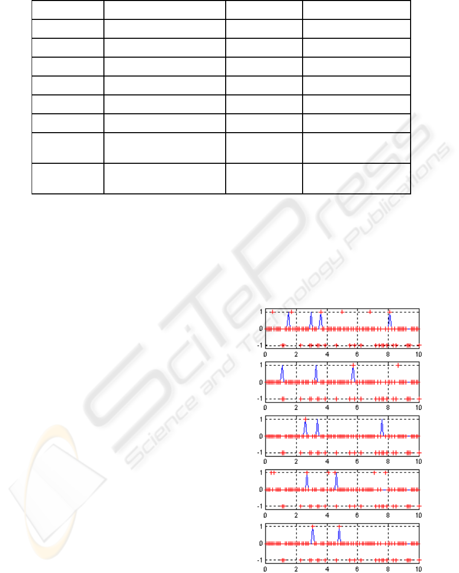
Table 2: Correspondence between syndromes and coset leaders for PN2.
Syndromes Errors of weight 1 Syndromes Errors of weight 1
(-1 0 0 1 0)
T
(1 0 0 0 0 0 0 0 0)
T
(1 0 0 0 0)
T
(0 0 0 0 1 0 0 0 0)
T
(1 0 0 -1 0)
T
(-1 0 0 0 0 0 0 0 0)
T
(-1 0 0 0 0)
T
(0 0 0 0 -1 0 0 0 0)
T
(0 1 -1 0 0)
T
(0 1 0 0 0 0 0 0 0)
T
(0 1 0 0 0)
T
(0 0 0 0 0 1 0 0 0)
T
(0 -1 1 0 0)
T
(0 -1 0 0 0 0 0 0 0)
T
(0 -1 0 0 0)
T
(0 0 0 0 0 -1 0 0 0)
T
(1 -1 1 -1 1)
T
(0 0 1 0 0 0 0 0 0)
T
(0 0 1 0 0)
T
(0 0 0 0 0 0 1 0 0)
T
(-1 1 -1 1 -1)
T
(0 0 -1 0 0 0 0 0 0)
T
(0 0 -1 0 0)
T
(0 0 0 0 0 0 -1 0 0)
T
(0 0 0 1 0)
T
(0 0 0 1 0 0 0 0 0)
T
(0 0 0 0 1)
T
(0 0 0 0 0 0 0 1 0)
T
(0 0 0 0 0 0 0 0 1)
T
(0 0 0 -1 0)
T
(0 0 0 -1 0 0 0 0 0)
T
(0 0 0 0 -1)
T
(0 0 0 0 0 0 0 -1 0)
T
(0 0 0 0 0 0 0 0 -1)
T
Simulations for on – line estimation of the
transitions firing are provided with figure 5. In these
simulations, a measurement error ratio of 0.1 is
supposed to be associated to each place (i.e. a
probability of 0.1 that the marking variation of each
place is biased). Transitions are assumed to fire with
stochastic firing periods (exponential distribution) of
mean value equal to 1 TU. All simulations indicate
that complexity of algorithm b is not a limitation for
real time applications. For the example PN2, the
total CPU time for algorithm b is less than 5 TU for
a simulation of 100 TU with a sampling period of 0.1
TU. This means that the average duration for each
cycle of algorithm is approximatively 20 times less
than the sampling period. The miss estimation rate
for b is about 32% in comparison with a that has a
rate of 60% and the wrong estimation rate is about
8% for b in comparison with a that has a rate less
than 1%. Let us mention that the large number of
miss estimation (even if measurement is unbiased) is
due to the small Hamming distance of W (d = 2). For
this reason numerous unbiased measurements of the
marking variation are considered as suspicious and
not used for estimation.
6 CONCLUSIONS
The investigation of diagnosis methods for discrete
event systems shows that Petri nets is efficient not
only to model the considered systems but also to
support the diagnosis methods. Several approaches
can be used in order to check diagnosability, to
select sensors and to work out diagnosers. As a
conclusion it is important to notice the great effort,
observed this last years to develop and improve
diagnosis methods for DES. The use of the coding
theory plays an important role in that development.
As long as it is suitable to detect and correct
measurement errors in the marking error variation.
The main drawback is the strong dependence of the
method to the algebraic properties of the incidence
matrix.
Figure 5: On – line firings estimation with algorithm b for
the transitions T
1
to T
5
of PN2 (number of firings, full
line: correct value; cross: estimated value; estimated value
= -1 means miss estimation) in function of time (TU).
DIAGNOSIS OF DISCRETE EVENT SYSTEMS WITH PETRI NETS AND CODING THEORY
21

The method can be improved by incorporating
additive places into Petri nets models. Taken into
account the past sequence of events is another
perspective to improve the efficiency of the method.
But, the main challenge is, from our point of view,
to take advantages from many important
contributions that have been proposed for
continuous systems. To build a bridge from
continuous variable systems to DES theories
remains one of the most promising issues for the
next years.
REFERENCES
Askin R.G., Standridge C. R. (1993). Modeling and
analysis of Petri nets, John Wiley and sons Inc.
Berlekamp R.E. (1984). Algebraic coding theory, Laguna
Hills, CA, Aegean Park.
Blanke M., Kinnaert M., Lunze J., Staroswiecki M.
(2003). Diagnosis and fault tolerant control, Springer
Verlag, New York.
Cassandras C.G., Lafortune S. (1999). Introduction to
discrete event systems, Kluwer Academic Pub.
David R., Alla H. (1992). Petri nets and grafcet – tools for
modelling discrete events systems, Prentice Hall,
London.
Lefebvre D., El Moudni A. (2001). Firing and enabling
sequences estimation for timed Petri nets, Trans. IEEE
- SMCA, vol. 31, no.3, pp. 153- 162.
Lefebvre D., Delherm C. (2007). Fault detection and
isolation of discrete event systems with Petri net
models, Trans. IEEE – TASE, vol. 4, no. 1, pp. 114 – 118.
Lefebvre D. (2008). Firing sequences estimation in vector
space over Z3 for ordinary Petri nets, , accepted for
publication in Trans. IEEE – SMCA.
Li L., Hadjicostis C. N. Sreenivas R. S. (2004). Fault
Detection and Identification in Petri Net Controllers,
Proc. IEEE-CDC04, pp. 5248 – 5253, Atlantis,
Paradise Island, Bahamas.
Ramirez-Trevino A., Ruiz-Bletran E., Rivera-Rangel I.,
Lopez-Mellado E. (2007). Online Fault Diagnosis of
Discrete Event Systems. A Petri Net-Based Approach,
Trans. IEEE – TASE, vol. 4, no. 1, pp. 31-39.
Rausand M., Hoyland A. (2004). System reliability theory
: models, statistical methods, and applications, Wiley,
Hoboken, New Jersey.
Ren H., Mi Z. (2006). Power system fault diagnosis
modeling techniques based on encoded Petri nets,
Proc. IEEE Power Engineering Society General
Meeting.
Sampath M., Sengupta R., Lafortune S., Sinnamohideen
K., Teneketzis D. (1995). Diagnosibility of discrete
event systems, Trans. IEEE-TAC, vol. 40, no.9, pp.
1555- 1575.
Silva M., Recalde L. (2004). On fluidification of Petri
Nets: from discrete to hybrid and continuous models,
Annual Reviews in Control, vol. 28, no. 2, pp. 253-266.
Ushio T., Onishi I., Okuda K., (1998). Fault detection
based on Petri net models with faulty behaviours,
Proc. IEEE – SMC98, pp 113-118.
Van Lint J.H. (1999). Introduction to Coding Theory,
Graduate Texts in Mathematics, vol. 86, Springer
Verlag.
Wu Y., Hadjicostis N. (2002). Non-concurrent fault
identification in discrete event systems using encoded
Petri net states, Proc. IEEE – CDC02, vol. 4, pp4018-
4023.
Wu Y., Hadjicostis N. (2005). Algebraic approaches for
fault identification in discrete event systems, Trans.
IEEE - TAC, vol. 50, no. 12, pp. 2048 – 2053.
ICINCO 2008 - International Conference on Informatics in Control, Automation and Robotics
22