TOWARDS THE ESTIMATION OF CONSPICUITY WITH VISUAL
PRIORS
Ludovic Simon, Jean-Philippe Tarel and Roland Br´emond
Laboratoire Central des Ponts et Chausses (LCPC), 58 boulevard Lefebvre, Paris, France
Keywords:
Machine learning, Image processing, Object detection, Human vision, Road safety, Conspicuity, Saliency,
Visibility, Visual performance, Evaluation, Eye-tracker.
Abstract:
Traffic signs are designed to be clearly seen by drivers. However a little is known about the visual influence of
the traffic sign environment on how it will be perceived. Computer estimation of the conspicuity from images
using a camera mounted on a vehicle is thus of importance in order to be able to quickly make a diagnosis
regarding conspicuity of traffic signs. Unfortunately, our knowledge about the human visual processing system
is rather incomplete and thus conspicuity visual mechanisms remain poorly understood. A complete model for
conspicuity is not known, only specific features are known to be of importance. It makes sense to assume that
an important task for drivers is to search for traffic signs. We therefore propose a new paradigm for conspicuity
estimation in search tasks based on statistical learning of the visual features of the object of interest.
1 INTRODUCTION
Not all traffic signs are seen by all drivers, despite the
fact that traffic signs are designed to attract driver’s
attention. This may be explained by different fac-
tors, one is that the conspicuity of the missed traf-
fic sign is too low. The conspicuity is the degree to
which an object attracts attention with a given back-
ground, when the observer is performing a given task.
This problem raises the question of how to estimate
the conspicuity of traffic signs along a road network.
Indeed, one may wish to design a dedicated vehicle
with digital cameras, which will be able to diagnose
traffic signs conspicuity along a road network. The
development of such a kind of system faces a difficult
problem: the model of conspicuity is only partially
known, due to our relatively limited, although grow-
ing, knowledge of the human visual system (HVS).
As explained in (CIE137, 2000), only features which
account in the conspicuity are known. This is mainly
due to the fact that measuring human attention is sub-
ject to many difficulties, even with eye-tracking.
The paper is organized as follow. First, we present
previous approaches which are connected to the prob-
lem, and explain why a new approach is requested.
Then a original approach is proposed. In section 3,
we describe our particular implementation of the pro-
posed approach. Finally, in the last two sections ex-
periments using an eye-tracker are described.
2 THE NEED FOR A NEW
APPROACH
In (Itti et al., 1998), the most popular computational
model for conspicuity was proposed. This model is
mainly based on the modeling of the low levels of
the HVS. Given any image, the algorithm computes
a so-called saliency map. Saliency maps were tested
with success in (Underwood et al., 2006), when the
observer task is to memorize images. But it was also
shown that when the task is to search for a particular
object, this model is no longer valid.
We ran experiments, described in (Bremond et al.,
2006; Simon et al., 2007), in order to test saliency
maps in a driving context, where the observer was
asked whether he would brake in front of a road im-
age. We concluded that the saliency map model is not
valid in such a situation. This is illustrated by figure 1
323
Simon L., Tarel J. and Brémond R. (2008).
TOWARDS THE ESTIMATION OF CONSPICUITY WITH VISUAL PRIORS.
In Proceedings of the Third Inter national Conference on Computer Vision Theory and Applications, pages 323-328
DOI: 10.5220/0001083503230328
Copyright
c
 SciTePress

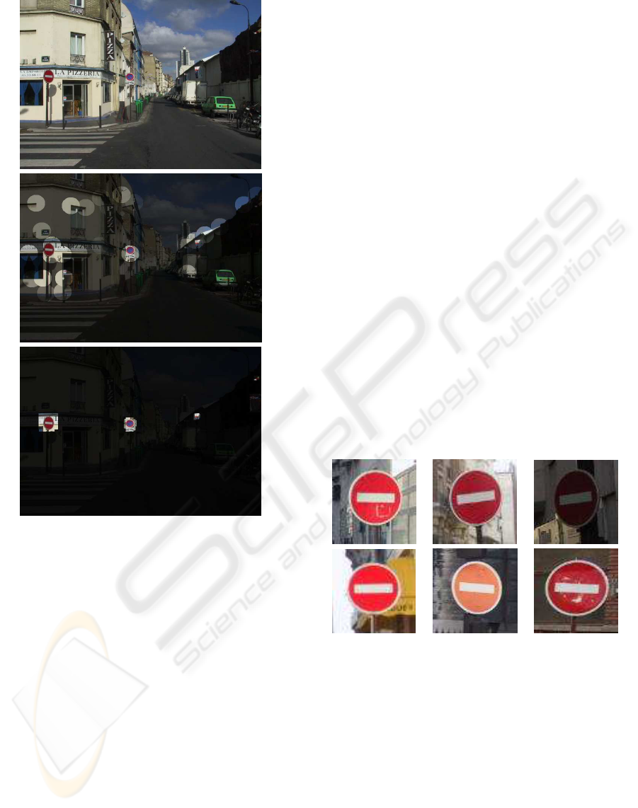
Figure 1: Top: the original image. Middle: saliency map
using (Itti et al., 1998). Bottom: proposed conspicuity map.
which shows in the middle the saliency map obtained
on the top road image. For sure, a driver will not look
at the sky and at the buildings, contrary to what was
predicted. The explanation is that in the driving con-
text, the involved tasks are not pure bottom-up tasks
as it is assumed in the saliency map model. Indeed,
this model does not take into account any prior in-
formation about the object or the class of objects of
interest for the task.
Other models of conspicuity in images with pri-
ors, (Navalpakkam and Itti, 2005) and (Sundstedt
et al., 2005), were later proposed. However, these
models are mainly theoretical rather than computa-
tional.
The previous discussion illustrate the needs for
new models of the conspicuity related to the observer
task. An interesting contribution along these lines
is (Gao and Vasconcelos, 2004), where a computa-
tional model of the so-called discriminant saliency is
proposed. In this model the observer task is to recog-
nize if a particular object is present, knowing the set
of possibly appearing objects. It is based on the se-
lection of the features that are the more discriminant
for the recognition. The image locations containing
a large enough amount of selected feature is consid-
ered as salient. In our opinion, the feature selection
as proposed in (Gao and Vasconcelos, 2004) will not
be able to tackle complicated situations where a class
of object may have very variable appearances. In-
deed, the dependencies between features are assumed
not informative. For instance, the color will be the
selected feature to distinguish a red balloon from a
white spherical lamp, the shape will be the selected
feature to distinguish a red balloon from a red desk
lamp, but the difficulty comes when it is necessary to
distinguish a red balloon from the two previous lamps
simultaneously.
In the driving context, an important task is to wait
for the arrival of traffic signs. Our goal is thus to cap-
ture accurately the priors a human learn on the appear-
ance of the object interesting for the task. By object,
we mean both a single particular object such as a ”no
entry” sign, and a set of objects such as path signs. We
thus decided to rely on statistical learning algorithms
to capture priors on object appearance, as previously
sketch in (Simon et al., 2007).
Figure 2: A few positive samples of the ”no entry” sign
learning databases.
The learning is performed from a set of positive and
negative examples. Each example is represented by
an input vector. Positive feature vectors are samples
of the appearance of the object of interest, when neg-
ative feature vectors are samples of the appearance
of the background. From this set, called the learn-
ing database, the learning algorithm is able to infer
the frontierthat splits the feature space into non-linear
parts associated to the object of interest and parts as-
sociated to the background. It is the so-called classifi-
cation function. Once the learning stage is performed,
the resulting classifier can be used to decide if the ob-
VISAPP 2008 - International Conference on Computer Vision Theory and Applications
324

ject of interest appears within any new images or new
image windows.
One advantage of the proposed approach is that
the learning algorithm can be also used for building a
detection algorithm of the object of interest. We now
assume that the learning algorithm is able not only to
estimate the class of any new image but also the con-
fidence it has in the estimated result. The conspicuity
of the object of interest within a complex background
image is directly related to our facility to detect it.
The proposed paradigm is thus to consider that the
image map of the conspicuity of the object of interest
is an increasing function of the map of how confident
the learning algorithm is in recognizing each location
as within the object of interest.
From a learning database of ”no entry” signs, see
figure 2, we built a ”no entry” sign detector by scan-
ning the windows of the input image, at different
sizes. The result is shown in bottom of figure 1, and
illustrates the advantages of the proposed approach
compared with a saliency map. It is clear from the lo-
cations selected as conspicuous, that the proposed ap-
proach outperforms bottom-up saliency models such
as Itti’s as long as road signs saliency while driving
is concerned. Indeed only ”no entry” signs or image
windows having similar colors than ”no entry” sign
are selected. As feature vector, 12
2
-bins color his-
togram in normalized rb space is used.
3 CONSPICUITY
COMPUTATIONAL MODEL
3.1 Learning Object Appearance
To perform road sign detection, we need to build
the classification function associated to the road sign
of interest, from the learning database. In the last
decade, several new and efficient learning algorithms
were proposed such as those derived using the ”Ker-
nel trick” (Sch¨olkopf and Smola, 2002). The best
known algorithm in this category is the so-called
Support Vector Machine (SVM) algorithm which
demonstrates reliable performances in learning ob-
ject appearances in many pattern recognition appli-
cations (Vapnik, 1999).
SVM is doing two-class recognition and consists
in two stages:
• Training stage: training samples containing la-
beled positive and negative images are used to
learn algorithm parameters. Each image or im-
age window is represented by vector x
i
with label
y
i
= ±1, 1 ≤ i ≤ ℓ. ℓ is the number of samples.
This stage consists in minimizing the following
quadratic problem with respect to parameters α
i
:
W(α) = −
ℓ
∑
i=1
α
i
+
1
2
ℓ
∑
i, j=1
α
i
α
j
y
i
y
j
K(x
i
,x
j
) (1)
under the constraint
∑
ℓ
i=1
y
i
α
i
= 0, where K(x,x
′
)
is a positive definite kernel. Usually, the above
optimization leads to sparse non-zero parameters
α
i
. Training samples with non-zero α
i
are the so-
called support vectors.
• Testing stage: the resulting classifier is applied to
unlabeled images to decide whether they belong
to the positive or the negative class. The label of
x is simply obtained as the sign of the classifier
function:
C(x) =
ℓ
∑
i=1
α
i
y
i
K(x
i
,x) + b (2)
where b is estimated using Kuhn-Tucker condi-
tions during training stage, after α
i
computation.
Using the scalar product as kernel leads to linear dis-
crimination. Using other kernels allows to take into
account the non-linearityof the boundaryin X by per-
forming an implicit mapping of X towards a space of
higher dimension.
In practice, we have build a learning database
for ”no entry” signs, see samples in figure 2 with a
set of 177 positive and 106139 negative feature vec-
tors. Cross-validation is used to select the kernel
and regularization parameters. When Laplace ker-
nel K(x,x
′
) = exp(−kx− x
′
k) is used, 28 positive and
11483 negative support vectors are selected. When
triangular kernel K(x, x
′
) = −kx − x
′
k, see (Fleuret
and Sahbi, 2003), the number of support vectors is re-
duced and as a result training and testing stages are
20 times faster. Indeed, only 939 negative and 74
positive support vectors are selected. This can be ex-
plained by the fact that the value of K(x,x
′
) does not
go towards zero when x goes far from x
′
. This gives
triangular kernel better extrapolation propertieson the
negative part of the feature space which is of much
larger size than the positive part.
3.2 ”no entry” Sign Detection
For any new image, ”no entry” sign detection is per-
formed by squared window scanning and by testing
if the class value of the current window is positive:
C(x) > 0, x being the feature vector of the current win-
dow. Indeed, when the C(x) is higher than one, x is
within the positive class with high probability. Sim-
ilarly, when the C(x) is lower than minus one, x is
within the negative class with high probability. When
TOWARDS THE ESTIMATION OF CONSPICUITY WITH VISUAL PRIORS
325

the C(x) is between zero and one, x can be considered
as positive but without certitude. Similarly, when the
C(x) is between minus one and zero, x can be consid-
ered as negative.
The translation increment during the scanning in
horizontal and vertical direction is of
1
4
of the win-
dow size. Due to the perspective, signs are seen
with difference sizes in the images and thus scans
are performed at different selected scales (10 × 10,
16× 16, 20× 20, 30× 30, 40× 40, 60 × 60 windows
for 640× 480 pixels image).
3.3 Confidence Map
The proposed paradigm is implemented as a SVM
learning algorithm for modeling the appearance of the
object of interest and the conspicuity map is an in-
creasing function of how confident the SVM is in rec-
ognizing each location as containing the object of in-
terest. The increasing function being unknown, we
will assume in the following that it is simply the iden-
tity function. We hope to investigate this point with
experimental road sign saliency data in further work.
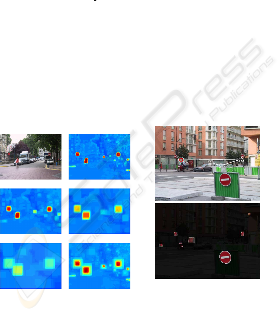
(a) (b)
(c) (d)
(e) (f)
Figure 3: The original image (a) and confidence maps ob-
tained at several scales: (b) 10×10, (c) 20×20, (d) 40×40,
(e) 60×60, and (f) the final confidence obtained by max se-
lection.
As explain before, one advantage of SVM is that the
obtained classifier is more informative that a binary
classifier. The value C(x) is computed and contains
information related to the confidence of the obtained
classification for each x. This is why, we assume that
the value C(x), when this value is positive, is the con-
fidence to be within the positive class.
At a given scale, we compute the confidence map
by affecting to the map the value of C(x) to all the
pixels of the window associated with feature vector x,
if C(x) > 0. If a pixel is associated to several confi-
dence values, due to window’s translation, the max-
imal value is selected. This map is called the confi-
dence map at a given scale, see Fig 3(b)(c)(d)(e). The
pixel’s maximal value is also selected to build a single
map from the maps at different scales, see Fig 3(f).
Following our paradigm, we define the search con-
spicuity map of the ”no entry” sign as the map of these
maximum confidences.
4 EYE TRACKING
Figure 4: On the top, the scan-path one subject searching for
”no entry” signs. Each circle represent a fixation. The dura-
tion is indicated in ms. The gaze starts at the image center.
Note that the sign on the bottom is missed. The image on
the bottom shows the predicted conspicuous locations using
color histogram in windows of different sizes.
After the description of our computational model
of conspicuity, a question is still open: what is the
correct choice for the feature vector type? To answer
VISAPP 2008 - International Conference on Computer Vision Theory and Applications
326

this question, we need reference data from the HVS.
In order to collect this reference data, we worked with
a remote eye-tracker, from SensoMotoric Instruments
(see http://www.smi.de/home/index.html ),
named iView X
TM
RED. The eye-tracker is used
to record positions and durations of the subjects’
fixations, on the images.
The subjects were asked to count for the ”no en-
try” signs in each image. An example of typical
scan paths is shown in figure 4. The initial focus is
set to the middle of the image by displaying a cen-
tered cross. The subjects only focused on two signs,
whereas they correctly count three signs. Indeed, sub-
jects do not need to focus on very conspicuous signs,
they may rely on parafoveal vision.
The locations predicted as conspicuous using the
proposed approach is again more consistent that what
is obtained using saliency map. Color histogram in
windows is used as feature. We experimented with
three subjects on the same images. Eye-tracker data
was also used to built average subjects’ fixations map
that can be used for as a reference when comparing
with confidence maps obtained using the SVM. Of
course, subjects also focused on objects relevant in
the task. These results are preliminary due to the re-
duced number of subjects. Extra psychophysical ex-
periments are requested to validate the proposedalgo-
rithm.
5 ON THE CHOICE OF FEATURE
Any image contains a great amount of information.
The question of the selection of a good feature is of
importance to fit as much as possible human search
conspicuity.
5.1 Small Versus Larger Windows
To tackle this question, we ran experiments to com-
pare confidence estimates obtained with different
kinds of features, from very local features to more
global ones. For each feature, the learning is per-
formed on 29 images of ”no entry” sign of various
aspects. Three kinds of features with different com-
plexities are selected: pixel colors, list of pixel colors
within a small window, color histograms in a larger
square window. 20 images of road scenes were tested
with different window size. In figure 5(a)(b)(c)(d),
the decision maps obtained with previous features are
shown. The original image is shown in figure 3(a). It
appears that the pixel colors and the list of pixel col-
ors within a small window are too local and thus leads
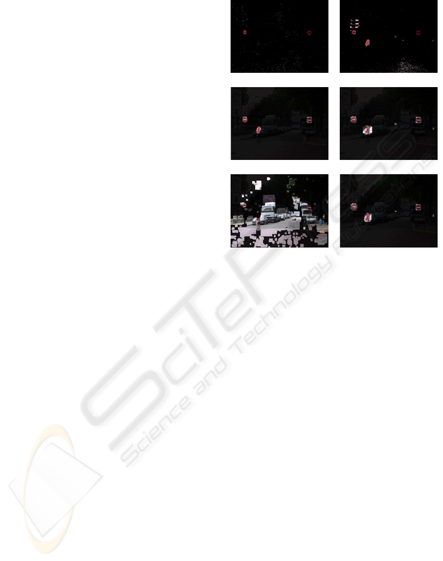
(a) (b)
(c) (d)
(e) (f)
Figure 5: Decision maps obtained on original image of fig-
ure 3(f), with different feature types: (a) pixel colors, (b)
list of pixel colors within a small window, (c) global 6
3
-
bins RGB color histograms in square window, (d) global
12
2
-bins rb color histograms in square window, (e) global
12-bins edge orientation histogram in a square window,
(f) global 12
2
-bins color and 12-bins edge orientation his-
tograms concatenated.
to maps with too many outlier. Color histograms pro-
vides the best results. The number of bins must not be
too reduced in order to not produce color mixture.
5.2 Color Versus Shape
We also ran experiments to see the relative impor-
tance of color and shape features. It is clear from fig-
ure 5(e) that decision maps obtained using the edge
orientation histogram is not correct. Shape alone is
not enough discriminative feature and must be used
in complement with color features, such as in fig-
ure 5(f) where 12
2
-bins color and 12-bins edge ori-
entation histograms were concatenated.
For more accurate comparison results, we build
ROC curves for each features, for different numbers
of bins. At first, we build two reference images for
each original image. The first reference is the mask
of ”No entry” signs. The second one is build from
the subjects’ fixations obtained with the eye-tracker
as explained in the previous section on original im-
age of figure 3(a). These two reference images are
TOWARDS THE ESTIMATION OF CONSPICUITY WITH VISUAL PRIORS
327

0 0.01 0.02 0.03 0.04 0.05
0
0.2
0.4
0.6
0.8
1
6−bins RGB
12−bins rb
12−bins OEH
12−bins rb+OEH
0 0.01 0.02 0.03 0.04 0.05
0
0.2
0.4
0.6
0.8
1
6−bins RGB
12−bins rb
12−bins OEH
12−bins rb+OEH
(a) (b)
0 0.005 0.01 0.015 0.02 0.025
0
0.2
0.4
0.6
0.8
1
6−bins RGB
12−bins rb
12−bins OEH
12−bins rb+OEH
0 0.005 0.01 0.015
0
0.2
0.4
0.6
0.8
1
6−bins RGB
12−bins rb
12−bins OEH
12−bins rb+OEH
(c) (d)
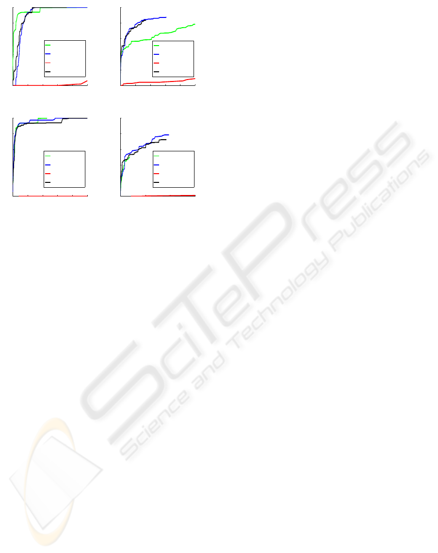
Figure 6: Comparison of ROC curves obtained on original
image of figure 3(a), with different feature types: 6
3
-bins
RGB color histogram, 12
2
-bins rb color histogram, 12-bins
edge orientation histogram, 12
2
-bins rb color and 12-bins
edge orientation histograms concatenated. In the first col-
umn, ground truth is ”No entry” signs, when in second col-
umn it is subjects’ fixations obtained by eye-tracker from 3
subjects. On the first line, Laplace Kernel is used when in
the second line it is the triangular kernel.
used as ground-truth for building two kinds of ROC
curves. The used parameter to draw the ROC curves
is the threshold on the confidence map for each fea-
ture. Four features were used: 6
3
-bins RGB color
histogram, 12
2
-bins rb color histogram, 12-bins edge
orientation histogram, 12
2
-bins rb color and 12-bins
edge orientation histograms concatenated. In figure 6,
the obtained ROC curves are displayed. On the left
column, the ground truth is ”No entry” signs, when
on the right column it is subjects’ fixations obtained
by eye-tracker from 3 subjects. Two different ker-
nels were used. On the first line, Laplace Kernel is
used when in the second line it is the triangular ker-
nel. In most of the cases, the best result is obtained
using 12
2
-bins rb color histogram.
6 CONCLUSIONS
We propose a new paradigm to define conspicuity in-
cluding visual priors on the object of interest. From
our preliminary experiments with subjects, this new
model seems to outperform the saliency map model.
We investigate the problem of choosing the right fea-
tures to describe a specific sign in images, and we
found that 12
2
-bins rb color histogram gives best per-
formances in most cases. We also investigate the in-
fluence of the choice of the kernel an we found that
triangular kernel leads to better and faster results. In
future work, we will continue to test our model using
the eye-tracker to validate the proposed paradigm and
to refine our conclusions.
REFERENCES
Bremond, R., Tarel, J.-P., Choukour, H., and Deugnier, M.
(2006). La saillance visuelle des objets routiers, un
indicateur de la visibilit´e routi`ere. In Proceedings of
Journ´ees des Sciences de l’Ing´enieur (JSI’06), Marne
la Vall´ee, France.
CIE137 (2000). The conspicuity of traffic signs in com-
plex backgrounds. In CIE137, Technical report of the
Commision Internationale de L’Eclairage (CIE).
Fleuret, F. and Sahbi, H. (2003). Scale-invariance of sup-
port vector machines based on the triangular kernel. In
Proceedings of IEEE International Workshop on Sta-
tistical and Computational Theories of Vision, Nice,
France.
Gao, D. and Vasconcelos, N. (2004). Discriminant saliency
for visual recognition from cluttered scenes. In NIPS.
Itti, L., Koch, C., and Niebur, E. (1998). A model of
saliency-based visual attention for rapid scene anal-
ysis. IEEE Transactions on Pattern Analysis and Ma-
chine Intelligence, 20(11):1254–1259.
Navalpakkam, V. and Itti, L. (2005). Modeling the influence
of task on attention. Vision Research, 45(2):205–231.
Sch¨olkopf, B. and Smola, A. (2002). Learning with Kernels.
MIT Press, Cambridge, MA, USA.
Simon, L., Tarel, J.-P., and Bremond, R. (2007). A new
paradigm for the computation of conspicuity of traffic
signs in road images. In Proceedings of 26th session of
Commision Internationale de L’Eclairage (CIE’07),
volume II, pages 161 – 164, Beijing, China.
Sundstedt, V., Debattista, K., Longhurst, P., Chalmers, A.,
and Troscianko, T. (2005). Visual attention for effi-
cient high-fidelity graphics. In Spring Conference on
Computer Graphics (SCCG 2005), pages 162–168.
Underwood, G., Foulsham, T., van Loon, E., Humphreys,
L., and Bloyce, J. (2006). Eye movements during
scene inspection: A test of the saliency map hy-
pothesis. European Journal of Cognitive Psychology,
18(3):321–342.
Vapnik, V. (1999). The Nature of Statistical Learning The-
ory. Springer Verlag, 2nd edition, New York.
VISAPP 2008 - International Conference on Computer Vision Theory and Applications
328