A NEW ALGORITHM FOR NAVIGATION BY SKYLIGHT
BASED ON INSECT VISION
F. J. Smith
School of Electronics, Electrical Engineering and Computer Science
Queens University, Belfast, N. Ireland
Keywords: Polarization, skylight, nav
igation, insect vision, POL, insect celestial map, robot, drone.
Abstract: Many insects can navigate accurately using the polarised light from the sky when the sun is obscured. They
navigate using
two different types of optical features: one is a set of three ocelli on the top of the head and
the second is a celestial compass based on several photoreceptors on the dorsal rims of the compound eyes.
Either feature can be used alone, but the dorsal rim receptors appear to be more accurate. Robots have been
built that navigate using three photoreceptors, or three pairs of orthogonally oriented photoreceptors, but
none has been designed which uses a full set of photoreceptors similar to those in the dorsal rim. A new
model of the function of the dorsal rim compass is proposed which relies on the four azimuths at which the
polarization angle χ = ±π/4. A simulation shows that this could provide an accurate navigational tool for a
robot (or insect) in lightly clouded skies.
1 INTRODUCTION
Due to the scattering of light within the earth’s
atmosphere, skylight is partially linearly polarized,
discovered by the Irish Scientist Tyndall (1869).
Two years later a full mathematical description of
the phenomenon was given by Lord Rayleigh (1871)
for the scattering by small particles in the
atmosphere (the particles we now know are air
molecules). That an insect can use this polarization
to navigate was first discovered in experiments with
bees by Karl von Frisch (1949).
It took another 25 years before the nature of the
insect’s celestial co
mpass began to be clarified
(Kirshfeld et al., 1975; Bernard and Wehner, 1977).
There are two different types of optical features
involved: the first is a set of ocelli, generally 3 in
number, on the top of the head (Goodman, 1970)
and the second depends primarily on a specialized
part of the insect compound eye, a comparatively
small group of ommatidia situated in the dorsal rim
area. Normally the ocelli and dorsal rim are
probably used together to navigate, in some way still
unknown, but experiments with desert ants (Fent and
Wehner, 1985) have shown that either feature can be
used successfully alone with the other blacked out.
It was also found in these experiments that the ocelli
are more erratic and less accurate for navigation than
the dorsal rim photoreceptors.
Further insight on the dorsal rim came from
R
udiger Wehner and co-workers working with
desert ants and bees (Labhart, 1980; Rossel and
Wehner, 1982; Wehner, 1997). It was found that
each ommatidium in the dorsal rim has two
photoreceptors with axes of polarization at right
angles to one another and each strongly sensitive to
the E-vector orientation of plane polarized light.
One of the axes of polarization of these ommatidia
has a fan shaped orientation that has been shown in
experiments to provide a map for the polarised sky,
a map which the insect can use as a compass
(Rossel, 1993). Recently this insect map of celestial
E-vector orientation has been found represented
within the central complex of the brain of an insect,
the cricket (Heinz and Homberg, 2007). We return
to this later.
Therefore much is known about this celestial
co
mpass and how it is represented within the brain.
However, relatively few contributions deal with the
physical mechanism underlying the compass, the
principal subject of this paper. Only one attempt has
been made (to our knowledge) to design a
navigational aid for a drone or robot based on this
compass; this uses only 3 pairs of photoreceptors
(Wehner,1997; Lambrinos et al, 1998), different
from the typical fan of 50 -100 pairs of receptors
185
J. Smith F. (2008).
A NEW ALGORITHM FOR NAVIGATION BY SKYLIGHT BASED ON INSECT VISION.
In Proceedings of the First International Conference on Bio-inspired Systems and Signal Processing, pages 185-190
DOI: 10.5220/0001068901850190
Copyright
c
 SciTePress

used by an insect or used in the design proposed
here. NASA has also built robots navigating by
skylight, but these use three photoreceptors with
different axes of polarization, probably the
underlying principle behind navigation by the ocelli
(NASA, 2005). Few details have been released on
the above systems, so comparison with our new
algorithm has not been possible.
In the following we first derive mathematical
expressions for the light intensities measured by the
photoreceptors, before showing how these can give
the direction of the sun.
2 THEORY
2.1 Measured Intensity
We begin with the assumption that the sky is blue,
with no cloud. Then it is well known (Rayleigh,
1871) that the light observed from any patch of sky
is partially polarised, with an elliptical profile for the
electric vector (although not elliptically polarised) in
which the major axis of the ellipse, is at right angles
to both the direction of the sun, represented by the
unit vector S, and to the direction of the observed
patch of sky, k’. We let k’ be one of three mutually
orthogonal vectors i’, j’ and k’, with i’ in the
direction of the major axis of the ellipse, and j’ in
the direction of the minor axis. The electric vector in
the direction of the major axis is often called the E-
vector. The angle which this makes clockwise in the
ellipse from the plane of the zenith, is called the
polarization angle, χ. In the ideal situation where all
of the light observed is scattered once only, the ratio
of the size of the minor axis to the size of the major
axis is known to be cos (θ) where θ is the angle
between S and k’.
Let E
S
be the scattered electrical vector being
observed. Then
]')sin()cos(' )[cos( jiE
S
φ
θ
φ
+= E
(1)
where E is the magnitude of the unpolarized electric
field. The angle
φ
determines the direction of the
vector within the ellipse; so it equals 0 when the
electric vector is parallel to the major axis.
When the partially polarised light enters an
ommatidium in the dorsal rim its intensity is
measured by two photoreceptors, each of which can
measure polarised light with parallel structures
called microvilli. The two directions of the
microvilli are at right angles to one another, and
define two orthogonal axes of polarization,
represented here by the orthogonal unit vectors i and
j, known as the X and Y photoreceptors. The third
mutually orthogonal vector, k, is in the same
direction as the observed patch of sky, so k = k’.
The angle which the vector i makes with the vertical
plane by rotation about k is called ξ.
We can now write the previous unit vectors in
Equation (1) in terms of i and j using the
transformation:
jij'
j
ii'
)cos()sin(
)sin()cos(
ξχξχ
ξ
χ
ξ
χ
−+−−=
−
+
−
+
=
(2)
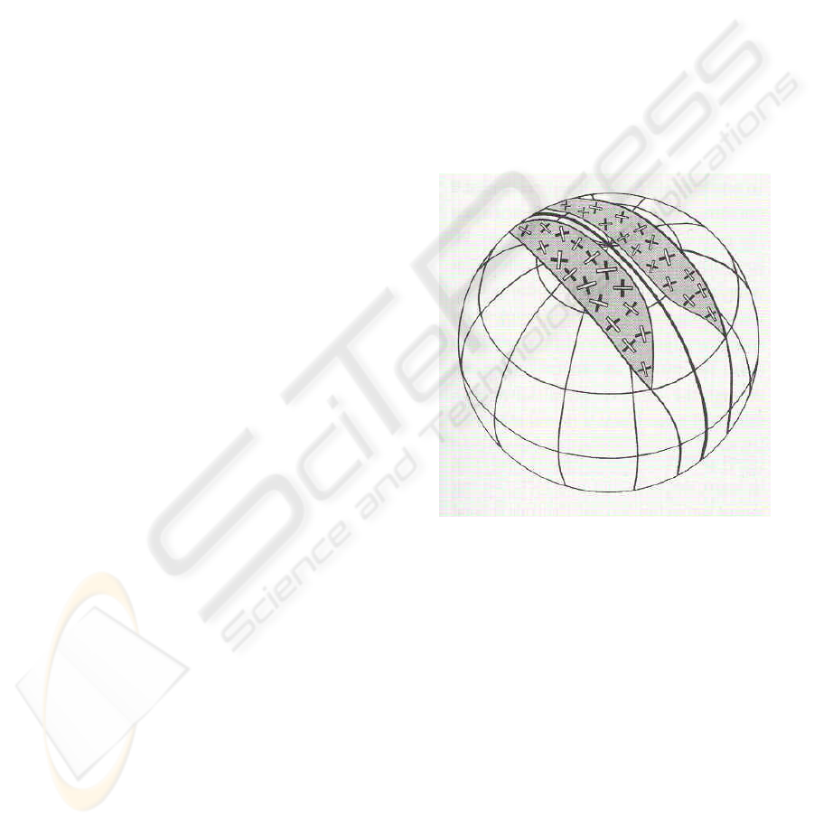
We look at the orientations of the microvilli
in the dorsal rim of the honey bee by Sommer
(1979), as copied in Figure 1. The fan shape of the
microvilli is apparent.
Figure 1: The paired orthogonal photoreceptors in the
dorsal rims of a bee. The Y photoreceptors are dark, the X
photoreceptors light (Sommer, 1979).
The observation of sky by the photoreceptors is
known to be contralateral, i.e. they observe the sky
on the opposite side of the head. An examination of
the figure shows that the axes of the X
photoreceptors are approximately parallel to the
meridians passing through the patches of sky being
observed contralaterally. The same approximate
parallel pattern was found in Desert Ants by Wehner
and Raber (1979). So we assume that the angle ξ
that the X polarization axis makes with this meridian
is always zero. This greatly simplifies our later
algorithm for a small insect brain.
We can now substitute for i’ and j’ from Eq.(2)
in Eq.(1) to obtain an expression for the partially
polarised vector E
S
in terms of the unit vectors i and
BIOSIGNALS 2008 - International Conference on Bio-inspired Systems and Signal Processing
186

j. For example, part of this is the magnitude, E
X
, of
the vector in the direction i to be measured by the
microvilli of the X photoreceptor:
(3)
()
)sin()cos()sin()cos()cos( φθχφχ −= E
X
E
However, each receptor can only measure a light
intensity, which is proportional to the summation of
the square of the amplitudes of the electrical vectors
for all angles
φ
. So, for receptor X, the measured
intensity, S
X
, is found by first integrating the square
of the amplitude in (3) over all angles and then
multiplying by a factor, 2R, which depends on terms
derived by Lord Rayleigh (1871) and on the
measuring capability of the photoreceptor.
Before writing down the result of the integration
we note that in the real world the sky is often not
always blue, but has a degree of haze or cloud
differing with direction. The light then entering the
ommatidia can be viewed as make up of two
components, one partly polarised as in the above
equations, and the second totally unpolarized due to
multiple scattering. We let U be the intensity of
unpolarized light measured by both photoreceptors.
Then we find
[
]
URES
X
+−= )(sin)(sin1
222
χθ
(4)
[
]
URES
Y
+−= )(cos)(sin1
222
χθ
(5)
It has been shown by Labhart(1988) that the POL
neuron at the bottom of each ommatidium of a
cricket records the difference between the two
signals, or rather the difference between the log of
the two signals, not the signals themselves; so the
signal recorded is
)()(
YXXY
SLnSLnS
−
=
(6)
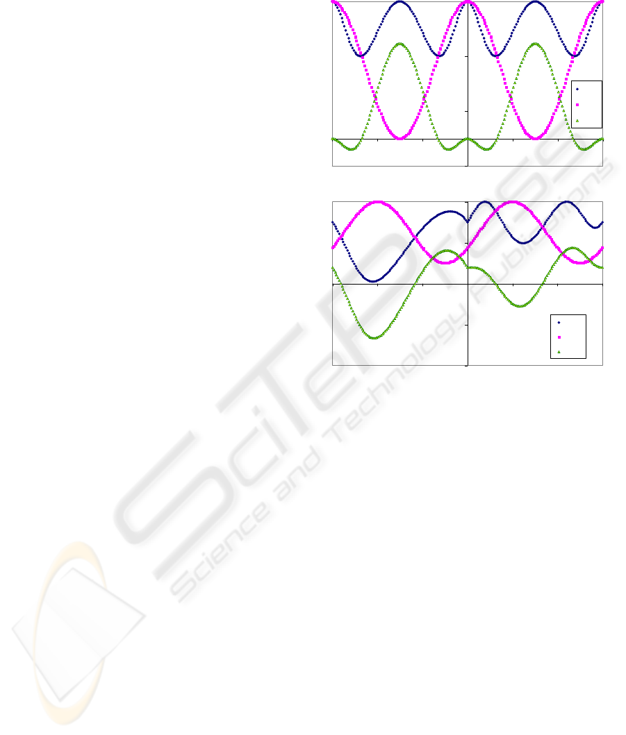
We set RE
2
= 1 in Figure (2) to illustrate the
variation in these signals as the azimuth angles of
the ommatidia vary.
Some of the above is known, but to proceed
further we need the polarization angle, χ. This
depends on the azimuth and elevation of the sun.
2.2 Solar Azimuth and Elevation
The angles θ and χ are related to the azimuth, a
s
, and
elevation, h
s
, of the sun. It is convenient to
introduce a third set of orthogonal axes, i’’, j’’ and
k’’ fixed on the earth, with i’’ and j’’ in the plane of
the ground and k’’ vertically upwards. For a
photoreceptor to find θ and χ we need also the
azimuth, a
o
, and elevation, h
o
, of the sky being
observed by the photoreceptor, i.e. towards the
centre of the patch of sky being observed. So we let
the unit vector i’’ point along the ground in this
direction.
-0.20
0.20
0.60
1.00
-180 -120 -60 0 60 120 180
Sx
Sy
Sxy
-1.00
-0.50
0.00
0.50
1.00
-180 -120 -60 0 60 120 180
Sx
Sy
Sxy
Figure 2: Illustration of the signals S
X
and S
Y
with U=0,
and S
XY
with U=1, as they vary with the azimuth of the fan
of observations, a
o
, measured from the central axis of the
insect. Top graph: h
s
=0, a
s
=0. Bottom: h
s
=30, a
s
=60. Note
that a
s
=a
o
at a maximum of S
Y
and that there are 4
azimuths where S
XY
=0, called zeros.
In terms of these new unit vectors we write the
vector pointing in the direction of the sun as S =
S
1
i’’ + S
2
j’’ + S
3
k’’ where
)sin(
);sin()cos(
);cos()cos(
3
2
1
s
oss
oss
hS
aahS
aahS
=
−=
−
=
(7)
We can write down two equations for the direction
of the sun. First we know that the vector k’, which
points at the observed patch of sky, makes an angle
θ relative to the direction of the sun, S. We also
know that the E-vector, in the direction represented
by the unit vector, i’, is at right angles to the plane
containing the solar unit vector, S, and the vector,
k’. So
(a) k’.S = cos(θ), and (b) i’.S = 0. (8)
We now express the unit vectors i’, describing
the E-vector, and k’ in terms of the new axes i’’, j’’
A NEW ALGORITHM FOR NAVIGATION BY SKYLIGHT BASED ON INSECT VISION
187

and k’’ fixed in the earth. Since k’ and k’’ are in the
same vertical plane it follows that
'
(9)
')sin('')cos(' kik
oo
hh +=
Noting that i’ is at right angles to k’ and that the
angle χ represents the orientation of the major axis
of the polarised light about the vector k’, it follows
that
(10)
'')sin()cos(]'')cos('')sin([' jkii χχ −+−=
o
h
o
h
Substitute and Equations (8a and b) become
)sin()sin()cos()cos()cos()cos(
s
h
o
h
s
ha
o
h += θ
(11)
)cos()sin()sin()cos()cos()sin()cos(
)sin()cos()cos(0
s
ha
s
ha
o
h
s
h
o
h
χχ
χ
−−
=
(12)
where a = a
s
– a
o
is the azimuth of the sun relative
to the azimuth of the observed sky.
A new unexpected equation was derived from
(11) and (12) after some analysis:
)cos()sin()cos()sin(
sos
haa −=
χ
θ
(13)
This can also be derived geometrically, or from the
relation k’ x S = sin(θ )i’. It simplifies the
calculation of the angle χ, although not its sign. But
more significantly, by substitution in (5), it changes
the expression for the measured intensity S
Y
:
[
]
)(cos)(sin1
222
sosY
haaRES −−=
(14)
This surprising result shows first that it is the same
for all elevations of the sky being observed and
second that, as the azimuth a
o
round the fan of
receptors varies, the position of the maximum value
of S
Y
gives a new measure for the azimuth of the
sun, for all elevations of the sun (see Figure 2).
Unfortunately, finding this maximum is not possible
if an insect is only measuring the difference in the
two log signals as in Equation (5). But this does not
stop a robot from using this strategy to find the solar
azimuth. But it can only be approximate as finding
the exact position of a maximum is always difficult.
2.3 A Precise Compass
We begin with a question - why have two orthogonal
photoreceptors, instead of one? A possibility is that
the contrast between the two signals is improved
near the maximum of one of them. Unfortunately
this is often obscured by the sin
2
(θ) term in
Equations (4) and (5), as evident in Figure (2). Also
we are left with the problem of the lack of precision
in the determination of the position of any
maximum, even enhanced.
The photoreceptors can only measure
intensities, but absolute intensities of light from the
sky are so variable that only comparisons between
intensities from the same region of the sky are
meaningful computationally. An example is the
ratio of the two intensities from the pair of
orthogonal receptors in one ommatidium. Although
this ratio can be measured accurately, the inclusion
of an unknown amount of unpolarized light, U,
makes it meaningful only when the two are equal
(the easiest factor to measure). Equating S
X
and S
Y
puts S
XY
= 0 in Equation (6), eliminates U, RE
2
and θ
and we get simply: .
)(cos)(sin
22
χχ =
This makes χ = ±π/4. So finding where S
XY
=0,
the quantity measured for each ommatidium, tells us
the precise azimuths a
o
where χ = ±π/4. We call this
a zero. An examination of Figure (2) shows that in
these two cases there are 4 zeros. Curves similar to
this were drawn for a range of solar azimuths and
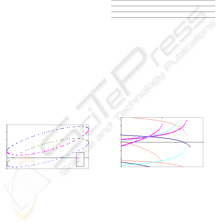
solar elevations and the zeros found. The zeros for
different solar azimuths are shown in Figure (3) for
one solar elevation. This and other examples show
that in almost all cases there are 4 zeros, usually 2
on either side of the head, but sometimes 4 on one
side and none on the other. When the elevation of
the sun is above the elevation of the observed patch
of sky there may be no zeros.
-180
-120
-60
0
60
120
180
0 60 120 180 240 300 360
a
s
a
o
Figure 3: Graph of azimuths, a
o
, of the observation at
which S
xy
= 0 (called zeros) for different values of the
solar azimuth, a
s
, at solar elevation, h
s
=30
o
. Zeros occur
when the two orthogonally polarized intensities are equal,
making χ=±π/4. There are usually 4 zeros, just enough to
uniquely define the azimuth and elevation of the sun.
We now show how we can use these 4 zero to make
a precise measurement of the sun’s position.
Noting that cos(χ) = 1 and sin(χ) = ±1 at the zeros,
Equation (12) becomes:
)tan()cos()sin(
)sin()cos(
soos
oos
hhaa
haa
=−±
−
(15)
BIOSIGNALS 2008 - International Conference on Bio-inspired Systems and Signal Processing
188

Solving this for a
s
, the azimuth of the sun, gives
δ
γ
±±=
os
aa
(16)
in which for each azimuth, there is a different γ
and δ given by γ = arccos(1/K) and δ =
arcsin(tan(h
o
a
s
)cos(h
o
)/K) where K
2
= 1+ sin
2
(h
o
).
The angle γ is fixed for each ommatidium; so it
might be stored as
γ
±
o
a
within the corresponding
neurons. It needs to be corrected with the angle δ
(unless the sun is on the horizon, when δ=0); but
this correction needs the observation of 4 zeros, as
discussed in the next section. If 4 zeros cannot be
observed because the region of observed sky is
restricted the insect can only use a
o
± γ, leaving an
error of δ. Such errors have been found in
experiments. So Equation (16) may be the
mathematical basis of at least part of the celestial
map in an insect brain.
The 4 alternatives in Equation (16) can also
regenerate exactly the results in Figure (3), but in an
inverted form. An example is shown in Figure (4).
In Figures (3) and (4) the elevations of the sky being
observed have been chosen to vary between 45
o
(at
azimuths 0
o
and 180
o
) and 80
o
(at azimuths ±90
o
).
However, these elevations are not critical: if all
ommatidia examine the sky at a constant high
elevation the algorithm described below is still valid
and the curves in Figures (3) and (4) all become
straight lines. There are still 4 zeroes, but none at
high solar elevations where sin(δ) > 1.
-90
-30
30
90
150
210
270
060120
180
s1
s2
s3
s4
a
s
a
o
Figure 4: Inverted graph of a
s
for positive a
o
calculated
using Equation (16) for h
s
=60
o
, showing the contribution
of the different ± combinations: s1: a
o
+γ +δ; s2: a
o
+γ
-δ; s3: a
o
–γ +δ; s4: a
o
–γ -δ.
We have built a simulator that can calculate the
position of the sun using the above equations. We
illustrate first with an example in which the
elevation of the sun is 30
o
and the solar azimuth is
20
o
; in this example the four zeros are at the
azimuths: a
o
= 53
o
, 145
o
, -5
o
, and -110
o
. For each
of these there are 4 alternatives given by Equation
(16), but an insect or a robot which is only
measuring intensities would not know which is
correct. Four alternatives for 4 zero angles makes a
total of 16 possibilities as in the array in Table 1.
Table 1: Example of array of 4 possible solar azimuths for
each of 4 zeros (where S
X
- S
Y
= 0) when the elevation of
the sun is 30
o
. Note that the correct azimuth (marked in
bold) is found once in each of the four rows corresponding
to the four zeros. This occurs only for the correct solar
elevation.
Zeros
γ+δ +γ-δ –γ+δ –γ-δ
52 180
20
85 -75
145 -89 125 165
20
-5 131
20
-31 -142
-110
20
-148 -72 120
So the algorithm is simple:
1. find the 4 zeros where S
X
= S
Y
;
2. obtain for each the two angles
γ
±
o
a
;
3. choose a possible solar elevation;
4. find the 4 possible azimuths for each zero
from Equation (16) and put in an array of
16 angles (as in the example);
5. scan the array for one angle in all 4 rows,
within a small tolerance (e.g. 1 degree). If
found, it is the solar azimuth;
6. if not found, increase the elevation (e.g. by
1 degree) and return to step 3.
Figure (5) shows how this algorithm converges to
the correct result for the example in Table 1.
-90
-60
-30
0
30
60
90
0 30609
hs
as
0
Figure 5: Graph showing, as the solar elevation h
s
varies,
how four of the elements in the 16 array elements in Table
1 converge on the correct result at the solar azimuth
a
s
=20
o
when h
s
=30
o
. (Only half of the graph is shown.).
Simulations with about 1000 examples have shown
that this algorithm succeeds is almost every case
with no ambiguity within a tolerance of 1 degrees.
Occasional errors or failure occur only at low or
high solar elevations (< 3
o
or > h
o
). Four zeros are
needed: three zeros give a typical 40% error rate.
The algorithm takes only a page of code, and once it
is given the positions of the 4 zeros it calculates the
A NEW ALGORITHM FOR NAVIGATION BY SKYLIGHT BASED ON INSECT VISION
189

solar azimuth in less than a second on a PC. It can
easily be built into the processor of any robot.
Besides the accuracy of the method it has the
advantage that it gives the solar azimuth anywhere
within 360
o
, with no ambiguity of π as in some other
algorithms. It is partially independent of
environmental conditions since some ommatidia
may be looking at blue sky while others are looking
at lightly clouded sky. The position of the zeros is
unchanged as long as a polarization pattern is
detectable below the cloud, which is more likely for
ultraviolet light detectors (Pomozi et al., 2001).
So the greatest difficulty in building a skylight
compass for a robot based on this algorithm is the
detection of the four zeros. One design uses an array
of about 100 pairs of orthogonal photoreceptors in a
circle round the robot. The problem is that each pair
would have to observe a patch of sky with an
accurate azimuth; the elevation, due to Equation
(14), would be less critical. In another design the
robot has one accurate pair of photoreceptors which
is rotated continually through 360
o
(like radar)
measuring the azimuth as it moves at a constant high
elevation (e.g. 70
o
).
3 CONCLUSIONS
We have shown that an accurate celestial compass
for a robot can be built round the principle of finding
4 zeros in the differences between the two signals
obtained from pairs of orthogonally polarised
photoreceptors. The algorithm was derived from
published studies on the anatomy of insect eyes and
on published experiments with insect navigation. In
particular Equation (16) explains why errors occur
when the view of an insect is restricted. The
algorithm is also simple enough for the small brain
of an insect; so we believe that the algorithm, or
something like it, is part of the celestial compass
within the brain of an insect.
At the heart of the algorithm are searches in
arrays of exactly 16 elements as in Table 1. So we
might expect evidence for this within the brain of an
insect. It is interesting to note that a topographic
representation of E-vector orientation has been
found to underlie the columnar organisation of the
central complex of the brain of a locust, and this
consists of stacks of arrays, each composed of a
linear arrangement of 16 columns (Heinze and
Homberg, 2007).
REFERENCES
Bernard, G D, Wehner, R, 1977. Functional similarities
between polarization vision and color vision, Vision
Res., 17, 1019-28.
Fent, K, Wehner, R, 1985. Ocelli: A celestial compass in
the desert ant Cataglyphis, Science, 228, 192-4.
Goodman, L. J., 1970. The structure and function of the
insect dorsal ocellus. Adv. Insect Phys., 7, 97-195.
Heinze, S, Homberg, U, 2007. Maplike Representation of
Celestial E-Vector Orientations in the Brain of an
Insect, Science, 315, 995-7.
Kirschfeld, K, Lindauer, M, Martin,H, 1975. Problems in
menotactic orientation according to the polarized light
of the sky, Z. Naturforsch, 30C, 88-90.
Labhart, T, 1980. Specialized Photoreceptors at the dorsal
rim of the honeybee’s compound eye: Polarizational
and Angular Sensitivity, J Comp. Phys., 141, 19-30.
Labhart, T, 1988. Polarised-opponent interneurons in the
insect visual system, Nature, 331, 435-7.
Lambrinos, D, Maris, M, Kobayashi, H, Labhart, T,
Pfeifer, P, Wehner, R, 1998. Navigation with a
polarized light compass, Self-Learning Robots II: Bio-
Robotics (Digest 1998/248) IEE, London, 7/1-4.
NASA, 2005. www.nasatech.com/Briefs/Oct05/
NPO_41269.html
Pomozi, I, Horvath, G, Wehner, R., 2001. How the clear-
sky angle of polarization pattern continues underneath
clouds, J. Expt. Biol, 204, 2933-42.
Rayleigh, Lord, 1871. On the light from the sky, its
polarisation and colour, Phil Mag,, 41, 107-20, 274-9.
Rossel, S, 1993. Mini Review: Navigation by bees using
polarised skylight, Comp. Biochem. Physiol, 104A,
695-705.
Rossel, S, and Wehner, R, 1982. The bee’s map of the e-
vector pattern in the sky, Proc. Natl. Acad. Sci. USA,
79, 4451-5.
Sommer, E W, 1979. Untersuchungen zur topo-
graphischen Anatomie der Retina und zur
Sehfeldoptologie im Auge der Honigbiene, Apis
mellifera (Hymenoptera). PhD Thesis,Un.Zurich.
Tyndall, J, 1869. On the blue colour of the sky, the
polarisation of skylight, and on the polarisation of
cloudy matter, Proc. Roy. Soc., 17, 223.
Von Frisch, K, 1949. Die Polarisation des Himmelslichts
als Orientierender Faktor bei den Tanzen der Bienen,
Experientia, 5, 142-8.
Wehner, R, 1989. The hymenopteran skylight compass:
matched filtering and parallel coding, J Exp. Biol.,
146, 63-85.
Wehner, R, 1997. The Ant’s celestial compass system:
spectral and polarization channels, In Orientation and
Communication in Arthropods, Ed. M. Lehler,
Birkhauser, Berlag, Basel, Switzerland, 145-85.
Wehner, R, and Raber, F, 1979. Visual spatial memory in
desert ants, Cataglyphis bicolor (Hymenoptera:
Formicidae), Experientia, 35, 1569-71.
BIOSIGNALS 2008 - International Conference on Bio-inspired Systems and Signal Processing
190