
COMBINING NOVEL ACOUSTIC FEATURES USING SVM TO
DETECT SPEAKER CHANGING POINTS
∗
Haishan Zhong,
∗
David Cho,
∗†
Vladimir Pervouchine and
∗
Graham Leedham
∗
Nanyang Technological University, School of Computer Engineering, N4 Nanyang Ave, Singapore 639798
†
Institute for Infocomm Research, 21 Heng Mui Keng Terrace, Singapore 119613
Keywords:
Speaker recognition, Feature extraction, Feature evaluation.
Abstract:
Automatic speaker change point detection separates different speakers from continuous speech signal by utilis-
ing the speaker characteristics. It is often a necessary step before using a speaker recognition system. Acoustic
features of the speech signal such as Mel Frequency Cepstral Coefficients (MFCC) and Linear Prediction Cep-
stral Coefficients (LPCC) are commonly used to represent a speaker. However, the features are affected by
speech content, environment, type of recording device, etc. So far, no features have been discovered, which
values depend only on the speaker. In this paper four novel feature types proposed in recent journals and con-
ference papers for speaker verification problem, are applied to the problem of speaker change point detection.
The features are also used to form a combination scheme using an SVM classifier. The results shows that the
proposed scheme improves the performance of speaker changing point detection as compared to the system
that uses MFCC features only. Some of the novel features of low dimensionality give comparable speaker
change point detection accuracy to the high-dimensional MFCC features.
1 INTRODUCTION
The aim of speaker changing point detection (speaker
segmentation) is to find acoustic events within an au-
dio stream (e.g finding the speaker changing point
in the continuous speech files according to different
speakers’ characteristics). Automatic segmentation of
an audio stream according to speaker identities and
environmental conditions have gained increasing at-
tention. Since some speech files are obtained from
telephone conversations or recorded during meetings,
there are more than one person speaking in the audio
recordings. In such cases before performing speaker
recognition it is necessary to separate audio signal ac-
cording to different speakers. Features extracted from
a speech waveform are used to represent the charac-
teristics of the speech and speaker. Among the fea-
tures acoustic features are those based on spectro-
grams of short-term speech segments. However, the
feature values that represent a speaker also vary due
to speech content, environment, type of recording de-
vice, etc. So far no features have been discovered,
whose values only depend on the speaker. Also, dif-
ferent speech features contains different information
about a speaker: some features reflect a person’s vo-
cal tract shape while others may characterise the vocal
tract excitation source.
Generally there are three main techniques for de-
tecting the speaker changing points: decoder guided,
metric based and model based. In this paper, a
method using Support Vector Machines (SVM) to find
speaker changing point in a continuous audio file is
presented. SVM is a binary classifier that constructs a
decision boundary to separate the two classes. SVM
has gained much attention since the experimental re-
sults indicate that it can achieve a generalisation per-
formance that is greater than or equal to other clas-
sifiers, but requires less training data to achieve such
an outcome (Wan and Campbell, 2000). Speaker seg-
mentation can be treated as a binary decision task: the
system must decide whether or not a speech frame
has the speaker changing point. This study uses the
SVM for seeking speaker changing points by com-
bining commonly used acoustic features with several
novel acoustic features proposed recently. The novel
features have been recently proposed by different re-
224
Zhong H., Cho D., Pervouchine V. and Leedham G. (2008).
COMBINING NOVEL ACOUSTIC FEATURES USING SVM TO DETECT SPEAKER CHANGING POINTS.
In Proceedings of the First International Conference on Bio-inspired Systems and Signal Processing, pages 224-227
DOI: 10.5220/0001060402240227
Copyright
c
SciTePress
searchers for the problem of speaker recognition.
The paper is organised as follows: section 2
describes the speaker segmentation method with
Bayesian Information Criteria. In section 3 the fea-
ture extraction is described for each feature type. In
section 4 the structure of SVM speaker segmentation
is explained. Section 5 presents the experimental re-
sults and draws the conclusion.
2 SPEAKER SEGMENTATION
WITH BIC
A speaker changing point detection algorithm us-
ing Bayesian Information Criterion (BIC) is proposed
in (Chen and Gopalakrishnan, 1998). A speech signal
is divided into partially overlapping frames of around
30 ms length using a Hamming window. Extraction of
acoustic features is performed for each speech frame.
A sliding window with minimum size W
min
and max-
imum size W
max
shifted by F frames is used to group
several consecutive frames. For detail grouping al-
gorithm the reader may refer to (Chen and Gopalakr-
ishnan, 1998). Each segment contains a number of
frames and is represented by the corresponding acous-
tic feature vectors. A segment can be modelled as a
single Gaussian distribution. The distance between
consecutive segments is calculated based on variances
of the Gaussian distributions that model the segments
in the feature space. The variance BIC (Nishida and
Kawahara, 2003) was developed from BIC and used
to represent the distance between two speech seg-
ments represented as their feature vectors. Variance
BIC is formulated with the following function:
∆BIC
i
variance
= −
n
1
+ n
2
2
log
i
|Σ
0
|+
+
n
1
2
log
i
|Σ
1
| +
n
2
2
log
i
|Σ
2
|+
+ α
1
2
(d +
1
2
d(d +1))log(n
1
+ n
2
)
(1)
where Σ
0
, Σ
1
and Σ
2
are the covariance values of
the whole segment, the first segment and the second
segment respectively, n
i
is the number of frames for
the i-th segment, and d is the dimensionality of the
acoustic feature vectors. The larger the variance BIC
of two segments is, the larger is the probability that
there is a speaker changing point between these two
segments. A sliding window is used to calculate the
variance BIC value for the whole speech files (Chen
and Gopalakrishnan, 1998). Local maxima in vari-
ance BIC values of the whole speech are marked as
the speaker changing points.
When different acoustic features are used, there
will be different variance BIC values generated for
a speech file. These values can be used as features
forming feature vectors to be used for determining
speaker changing points. Fig. 1 shows the process of
generating a variance BIC vector after acoustic fea-
ture extraction. After the feature extraction for each
frame, the feature vector of each frame is used to cal-
culate the variance BIC values.
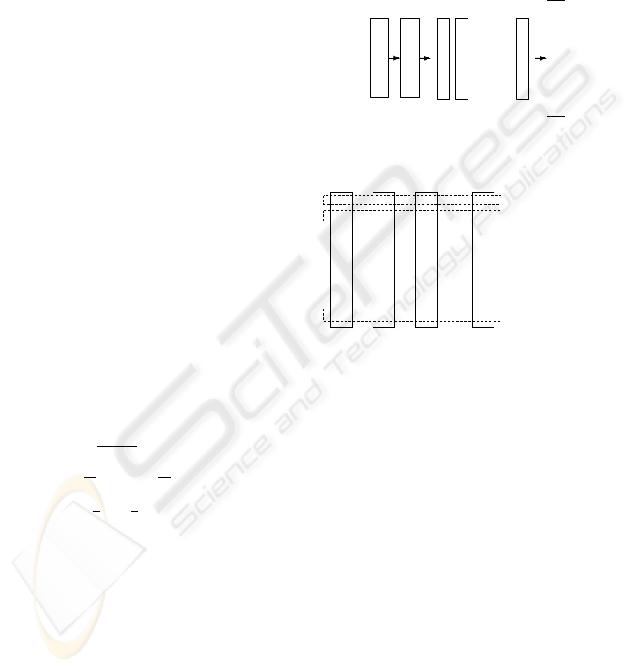
Audio signal
Acoustic features
Acoustic feature vectors
Frame 1
Frame 2
Frame n
…
Calculate variance BIC value
Figure 1: Generating variance BIC values for single type
acoustic features.
SVM feature vector for Frame 1
SVM feature vector for Frame 2
……….
SVM feature vector for Frame n
Feature 1 Feature 2 Feature 3 Feature n
BIC values
BIC values
BIC values
BIC values
Figure 2: Combination of variance BIC values generated
from different acoustic features into feature vectors.
Most of the acoustic features are of high dimen-
sionality, and simple concatenation of the feature vec-
tors will result in a feature vector of even higher di-
mensionality, which, in turn, will require too many
training samples to be trained reliably. Instead, in
the current study the variance BIC value is calculated
from each of the acoustic features as described above.
The BIC values calculated for the same frames using
different acoustic features form new feature vectors
are then used with the SVM classifier (Fig. 2).
3 EXTRACTION OF FEATURES
The features were extracted from speech sampled
at 16 kHz. Mel Frequency Cepstral Coefficients
(MFCC) (Oppenheim and Schafer, 2004) features
were used to calculate the variance BIC values.
MFCC vectors were extracted from 30 ms frames
without overlap. The feature values were normalised
by subtracting the mean and dividing by the standard
COMBINING NOVEL ACOUSTIC FEATURES USING SVM TO DETECT SPEAKER CHANGING POINTS
225
deviation. First order difference features were added.
In addition, several novel acoustic features were used
to calculate variance BIC values: Mel Line Spec-
trum Frequencies (MLSF) (Cordeiro and Ribeiro,
2006), Hurst parameter features (pH) (Sant’Ana et al.,
2006), Haar Octave Coefficients of Residue (HO-
COR) (Zheng and Ching, 2004), and features based
on fractional Fourier transform (MFCCFrFT).
FrFTMFCC
p
are extracted similarly to MFCC
with the only difference that the fractional Fourier
transform of order p is used in place of the inte-
ger one. Features of various orders p were tried
and FrFTMFCC
0.9
were chosen because they gave
the next highest speaker segmentation accuracy after
FrFTMFCC
1.0
, which are the conventional MFCC, as
measured by the F-score (see below).
MLSF are similar to Line Spectrum Frequencies
calculated from LP coefficients and were proposed in
the context of the speaker verification problem. A mel
spectrum was generated via Fast Fourier Transform
(FFT) and mel filter bank applied to 30 ms frames.
The inverse Fourier transform was applied to calcu-
late the mel autocorrelation of the signal, from which
MLSF features were then calculated via Levinson-
Durbin recursion. LP of order 10 was used. The fea-
ture values were normalised by subtracting the mean
and dividing by the standard deviation.
Hurst parameter is calculated for frames of a
speech signal via Abry-Veitch Estimator using dis-
crete wavelet transform (Veith and Abry, 1998). In the
current study a frame length of 60 ms was used, and
Daubechies wavelets with four, six, and twelve coef-
ficients were tried giving rise to pH
4
, pH
6
, and pH
12
features. The depth of wavelet decomposition was
chosen to be 5, 4, and 3 for pH
4
, pH
6
, and pH
12
corre-
spondingly, thus resulting in 5-, 4-, and 3-dimensional
feature vectors (Sant’Ana et al., 2006).
While LP coefficients are aimed at characteris-
ing the person’s vocal tract shape, information about
the glottal excitation source can be extracted from
the residual signal e
n
= s
n
+
∑
p
k=1
a
k
s
n−k
. Haar Oc-
tave Coefficients of Residue (HOCOR) features are
extracted by applying Haar transform to the residual
signal. In the current study the LP of order 12 was
applied to 30 ms frames. HOCOR
α
features of order
α 1, 2, 3, and 4 were extracted (Zheng and Ching,
2004).
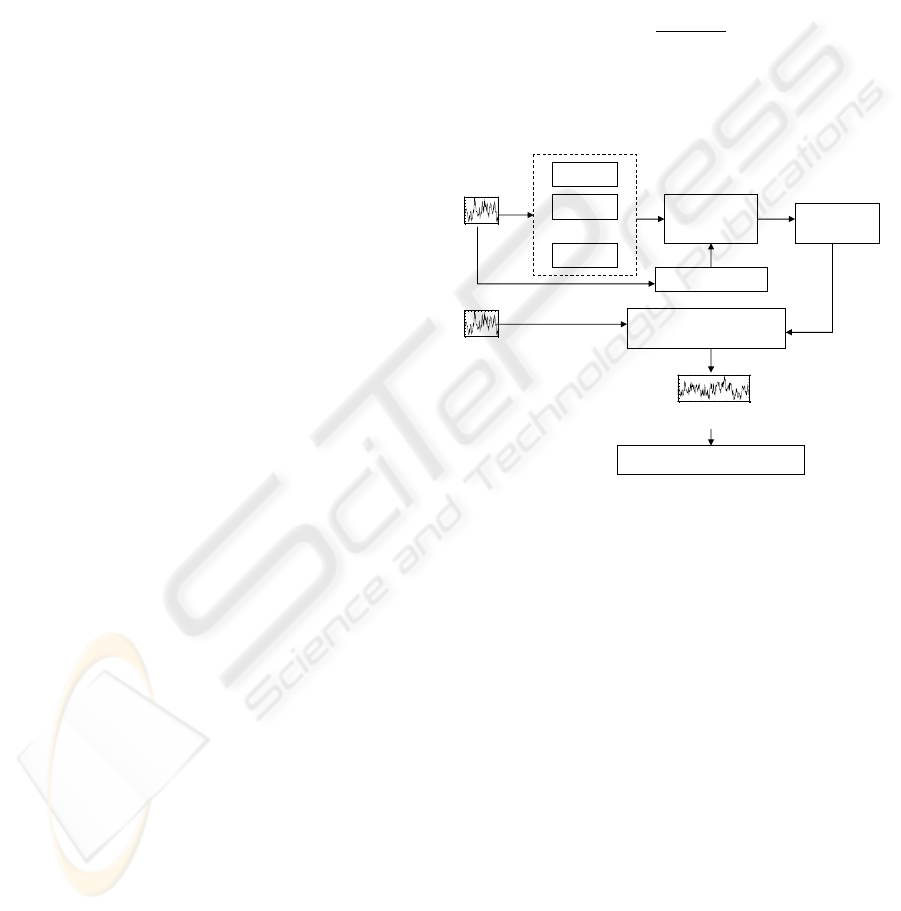
4 SVM SPEAKER
SEGMENTATION
Fig. 3 shows the structure of SVM speaker segmen-
tation. To be used in SVM the frames which contain
speaker changing point are labelled as −1, the frames
without speaker changing point are labelled as 1. The
acceptable error range of the found speaker chang-
ing points was chosen to be 1 second (Ajmera et al.,
2004), which means the frames that are half a sec-
ond before and after a speaker changing point are all
labelled as −1. The variance BIC values that are ob-
tained from different acoustic features are of different
order. To use them as features in SVM a linear scaling
is applied:
ˆ
f
j
i
=
f
j
i
−
h
f
i
i
σ
i
(2)
where i represent different features, j is the frame
number of the i-th feature,
f
j
is the mean value of
f
j
j
and σ
i
is its standard deviation.
Feature 1
Feature 2
Feature N
SVM
feature vector
Labelled speech
Training
SVM model
0 10 20 30 40 50 60 70 80 90 1 00
-0.04
-0.03
-0.02
-0.01
0
0.01
0.02
0.03
0.04
0.05
0 10 20 30 40 50 60 70 80 90 100
-0.04
-0.03
-0.02
-0.01
0
0.01
0.02
0.03
0.04
0.05
0 50 100 150 200 250 300
-0.06
-0.04
-0.02
0
0.02
0.04
0.06
0.08
Class values
Testing
SVM speaker segmentation
Find speaker changing points
…..
Figure 3: SVM speaker segmentation system.
The SVM classifier returns two values for each
frame that are related to the distance to the separat-
ing hyperplane (either of them can be monotonically
mapped into the conditional class probability). The
values sum to one and indicate to what extent the
frame belongs to class −1 (or 1). The −1 class value
is analysed to determine the true speaker changing
point. A peak search algorithm was used to deter-
mine the local maxima of −1 class value as we moved
along the frames. The peak searching algorithm uses
adaptive threshold in an attempt to eliminate small
peaks due to noise and find only true local maxima.
5 RESULTS AND CONCLUSION
The NIST HUB-4E Broadcast News Evaluation data
set was used in this study. The data was obtained
from the audio component of a variety of television
and broadcast news sources and each audio file con-
sist of approximately one hour of speech in English
BIOSIGNALS 2008 - International Conference on Bio-inspired Systems and Signal Processing
226
and includes the speech of several speakers in one au-
dio channel (Hub, 1997). To evaluate the performance
of the speaker changing point detection, two criteria
were used: the precision of speaker changing points
that were found and the number of missed changing
points. The precision indicates the percentage of true
turning points from the total number of turning points
that were found. The recall indicates how many of the
true turning points were missed. These two are com-
bined into an F-score. F-score indicates how good
a system is: it is high when both precision and re-
call values are high and low when either of them is
low (Nishida and Kawahara, 2003).
Table 1: F-score, precision and recall for different features
and their combination via SVM. d is the dimensionality of
the acoustic feature vectors.
Feature d F-score Precision Recall
MFCC 26 0.62 0.61 0.62
MLSF 10 0.42 0.29 0.80
pH
4
5 0.52 0.67 0.43
pH
6
4 0.53 0.67 0.44
pH
12
3 0.55 0.68 0.46
HOCOR
1
6 0.42 0.54 0.35
HOCOR
2
5 0.37 0.47 0.30
HOCOR
3
4 0.31 0.39 0.26
HOCOR
4
3 0.30 0.38 0.25
FrFTMFCC
0.9
12 0.61 0.73 0.56
SVM
1
10 0.64 0.72 0.58
SVM
2
6 0.65 0.75 0.58
Table 1 (except for the two bottom rows) shows
the speaker changing point detection results achieved
when different acoustic features were used to calcu-
late the variance BIC and the peak detection algorithm
was used to detect speaker changing points from the
BIC values. It is worth noticing that using pH features
gives F-scores comparable to those when MFCC fea-
tures are used, even though the dimensionality of fea-
ture vectors of pH features is far less than those of
MFCC. This suggests that pH features may be a bet-
ter choice when the training data set is small.
The features used for SVM combination 1
(SVM
1
) are the 10 variance BIC values resulted from
the 10 acoustic features. The results in Table 1 show
that the proposed SVM speaker changing point de-
tection scheme improves the speaker changing point
detection performance as compared to each of the
individual acoustic features, with a higher F-score
of 0.64. This means that other acoustic features,
which were originally proposed for speaker recogni-
tion problem, can be used for the problem of speaker
segmentation as well. Because of low both preci-
sion and recall values achieved on HOCOR features,
a combination of the acoustic features was attempted
without HOCOR features. The results (SVM
2
in Ta-
ble 1) were comparable with those of SVM
1
. How-
ever, elimination of any other acoustic features from
the combination degraded the speaker segmentation
performance.
This study demonstrates that the new features
do carry additional information about speaker dif-
ferences to MFCC features, and some of them also
have attractiveness because of their low dimensional-
ity. Further study may find better ways of how to in-
tegrate complimentary information about speaker dif-
ferences contained in the new features with traditional
features such as MFCC and LPCC.
REFERENCES
(1997). NIST HUB-4E Broadcast News Evaluation.
Ajmera, J., McCowan, I., and Bourlard, H. (2004). Robust
speaker change detection. IEEE Signal Process. Lett.,
11(8).
Chen, S. and Gopalakrishnan, P. (1998). Speaker, environ-
ment and channel change detection and clustering via
the Bayesian Information Criterion. In DARPA Speech
Recognition Workshop, pages 127–132.
Cordeiro, H. and Ribeiro, C. (2006). Speaker characteriza-
tion with MLSF. In Odyssey 2006: The Speaker and
Language Recognition Workshop, San Juan, Puerto
Rico.
Nishida, M. and Kawahara, T. (2003). Unsupervised
speaker indexing using speaker model selection based
on Baysian Information Criterion. In Proc. IEEE
ICASSP, volume 1, pages 172–175.
Oppenheim, A. and Schafer, R. (2004). From frequency to
quefrency: a history of the cepstrum. Signal Process-
ing Magazine, IEEE, (5):95–106.
Sant’Ana, R., Coehlo, R., and Alcaim, A. (2006). Text-
independent speaker recognition based on the Hurst
parameter and the multidimensional fractional Brow-
nian motion model. IEEE Trans. Acoust., Speech, Sig-
nal Process., 14(3):931–940.
Veith, D. and Abry, P. (1998). A wavelet-based joint estima-
tor of the parameters of long-range dependence. IEEE
Trans. Inf. Theory, 45(3):878–897.
Wan, V. and Campbell, M. (2000). Support vector machines
for speaker verification and identification. pages 775–
784.
Zheng, N. and Ching, P. (2004). Using Haar transformed
vocal source information for automatic speaker recog-
nition. In IEEE ICASSP, pages 77–80, Montreal,
Canada.
COMBINING NOVEL ACOUSTIC FEATURES USING SVM TO DETECT SPEAKER CHANGING POINTS
227
