SIMULATING REACTIVE/PASSIVE POSTURES BY MEANS OF
A HUMAN ACTIVE TORQUE HYBRID MINIMIZATION
I. Rodríguez
Department of Applied Mathematics and Analysis, University of Barcelona, Barcelona, Spain
R. Boulic
Virtual Reality Lab., Ecole Polytechnique Fédérale de Lausanne, Switzerland
Keywords: Virtual human poses, active muscle torque, passive resistive torque.
Abstract: In this paper we propose a hybrid approach minimizing the active torque produced by muscles groups at the
joint level. The proposed approach is hybrid in the sense that it combines the local knowledge of the
external torque induced by external forces such as gravity and exerted force, and the full knowledge of the
passive-resistive torque characteristics due to ligaments and connective tissues. The algorithm is exploited
within a context of posture adjustment when a muscle group reaches a critical fatigue level. It proposes a
target joint state that can be characterized as active or passive. The active solution, if it exists, can be further
characterized by a desired degree of active torque amplitude reduction (between 0 and 100%). In any cases
at least one passive solution exists; it relies on the passive/resistive torque appearing in the neighbourhood
of the joint limits.
1 INTRODUCTION
Postures and motions generated by the human body
are very difficult to simulate since it has so many
interrelated muscles that produce movement.
Muscles contractions are directly influenced by
physiological factors such as fatigue or
psychological factors such as the state of mind.
Biomechanical and biomedical studies have
modelled some of these factors (Kulig et al., 1984)
(Kumar, 1986). In Computer Animation, Multon
proposed a simulation environment where
biomechanicians could experiment on the motion
dynamics of a virtual arm (Multon, 1998). Komura
combined Delp’s musculoskeletal model (Delp,
1990) and Giat’s fatigue model (Giat et al., 1993) to
deal with full body character animations (Komura et
al. 2001).
The present paper is complementary to prior
studies in computer animation in the sense that we
investigate, at the joint level, how to reduce the
active torque as a function of an active or a passive
strategy. Indeed, this factor strongly influences the
postures adopted by individuals leading to reactive
or relaxed postures as recalled now. Early studies
showed that people resting with no immediate action
to do, tended to adopt asymmetrical (left/right body
side bears body weight) poses such as the pelvic
slouch (Evans, 1979). An asymmetrical posture is a
relaxed pose, incompatible with sudden responses.
For example, people waiting to be collected or
waiting for the bus. If there is a possibility of having
to do something, people adopt a symmetrical
standing (standing people such as police officers,
waiters, etc.). In an asymmetrical stance, the knee of
the supporting limb is fully extended and the thigh
fully adducted, therefore knee and hip joints finish
up hanging on their ligaments which produce
passive moment. This is also known as the
contraposto posture in sculpture (e.g. “David” of
Michelangelo).
Our hypothesis is that active torque, produced by
the muscle activation, can be reduced by means of
two strategies: either an active strategy searching for
a solution while staying in the mid-range of the joint
where the muscle efficiency is the highest, or a
passive one searching for the always existing
passive-resistive solution that compensates the
external torque in the neighborhood of the joint
5
Rodríguez I. and Boulic R. (2007).
SIMULATING REACTIVE/PASSIVE POSTURES BY MEANS OF A HUMAN ACTIVE TORQUE HYBRID MINIMIZATION.
In Proceedings of the Second International Conference on Computer Graphics Theory and Applications - AS/IE, pages 5-12
DOI: 10.5220/0002075700050012
Copyright
c
 SciTePress

limits. Considering these strategies allows to
generate a larger space of realistic postural solutions;
the active strategy achieves reactive poses while the
passive one produces relaxed poses.
The paper presents an initial evaluation of a
general algorithm of hybrid minimization of the
active torque under the quasi-static hypothesis. It is
illustrated on a simple case study (i.e. the elbow
joint) to characterize the various convergence
configurations arising from its specificity of
exploiting the local knowledge of the external torque
and the full knowledge of the passive torque
behavior.
2 ACTIVE TORQUE REDUCTION
SCHEME
Under the quasi-static hypothesis, the sum of all
torques is null for all joints. Therefore the joint
active torque τ
a
can be expressed as follows:
where, τ
p
and τ
e
represent, respectively, the current
passive and external joint torques. The external
torque τ
e
is produced by gravity and any other
external forces, while the passive torque τ
p
is due to
the resistance of the joint surrounding tissues
(ligaments and connective tissues) to be extended or
compressed. A null active torque is achieved when:
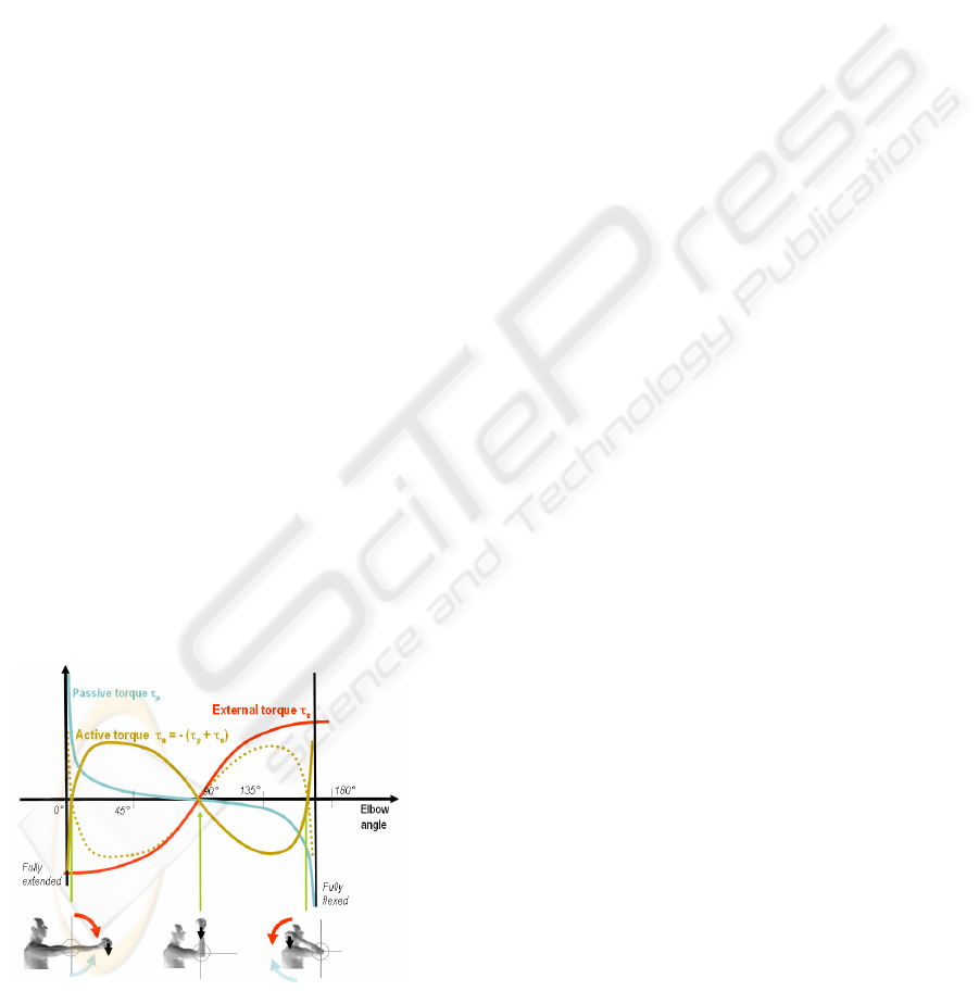
This is illustrated on Figure 1 where we have
three postures (photos) with a null τ
a
for the elbow
joint.
Figure 1: Frontal elbow case study highlighting the
passive torque (blue), the external torque (red), resulting
active torque (brown) and minus active torque (dotted
brown) under the quasi-static hypothesis. In this case, only
the elbow joint is varying.
2.1 Muscle Action Strategy
Our system introduces the muscle action strategy in
order to determine the influence of passive/resistive
torque (Hatze, 1997) in the active torque reduction
process.
An active strategy strives to find a solution close
to the mid-range of the joint where the muscle group
is efficient to produce its active torque,
τ
a
. Such a
region can be also characterized by a quasi-null
passive resistive torque (τ
p
≈0, see Figure 1).
The passive strategy only exploits the joint
passive torque to compensate the action of the
external torque. Such a solution is always in the
neighborhood of the joint limits, resulting in less
reactive/responsive muscles groups because muscles
forces are small even for a high degree of activation.
In the scenario from Figure 1, only the elbow
joint is allowed to move. Three postures with a null
active torque are highlighted (with a photo below).
The one in the central joint range is the active
solution as it maximizes the muscle activation
efficiency while the other two are purely
passive/resistive, hence less responsive.
2.2 Hybrid Algorithm
The proposed approach is hybrid in the sense that it
combines the local knowledge of the external torque
τ
e
and the full knowledge of the passive-resistive
torque characteristics τ
p
.
Indeed, in the general case, the number of
considered joints can be arbitrary large leading to
unknown variation of the external torque at the
individual joint level. In the quasi-static context we
can simply evaluate its current value τ
e
, by means of
the principle of the virtual works (Craig, 1986) and
its current first derivative, dτ
e
(section 3). As a direct
consequence, the algorithm we propose exploits only
a linear extrapolation of the external torque based on
this information.
On the other hand, we assume we know the
passive torque function τ
p
over the full joint range
from the Biomechanics literature (Esteki and
Mansour, 1996).
As a side remark, in the use-cases illustrating the
paper (Figure 1, Figure 10, Figure 12), the external
torque is induced by the gravity, and the only joint
that moves is the elbow. This allows to draw the
external torque function (i.e. the red curve); however
only the local knowledge of the external torque is
exploited in the result section.
In addition to the specification of the strategy
type - active vs passive - the active strategy selects
)(
epa
τ
τ
τ
+
−=
(1)
pe
ττ −=
(2)
GRAPP 2007 - International Conference on Computer Graphics Theory and Applications
6

its solution based on a normalized quantity called
the active torque decrease ratio R characterizing the
quality of the optimized active torque. We have:
where τ
a
represents the current active torque, τ
a_min
is
the estimated local minimum of the active torque
amplitude, when it exists, in addition to the null
global minima achieved with the passive strategy.
When τ
a_min
is null, a 100% of τ
a
decrease ratio is
achieved. This is the ideal case. In other less optimal
cases smaller values of R are achieved. For this
reason, the active strategy accepts a threshold level
R
min
on this quantity (potentially user-defined).
Whenever R is smaller than R
min
then the solution
provided by the active strategy is not accepted and
the algorithm switches to the always-existing
extremal passive solution. For example, a R
min
value
of 0.9 means that the user agrees to have down to
only 90% compensation because the remaining 10%
of active torque is a bearable amplitude. This favors
solutions lying in the mid joint range characterizing
a more reactive posture, even if they are not fully
optimal in terms of amplitude.
Table 1 details the algorithm providing the angle
θ
g
with reduced active torque. Its input is the current
joint state θ
c
, the active strategy boolean, the current
values of τ
e
, τ
p
and τ
a
, the current first derivative of
the external torque dτ
e
and of the passive torque dτ
p
(tabulated), and the threshold R
min
.
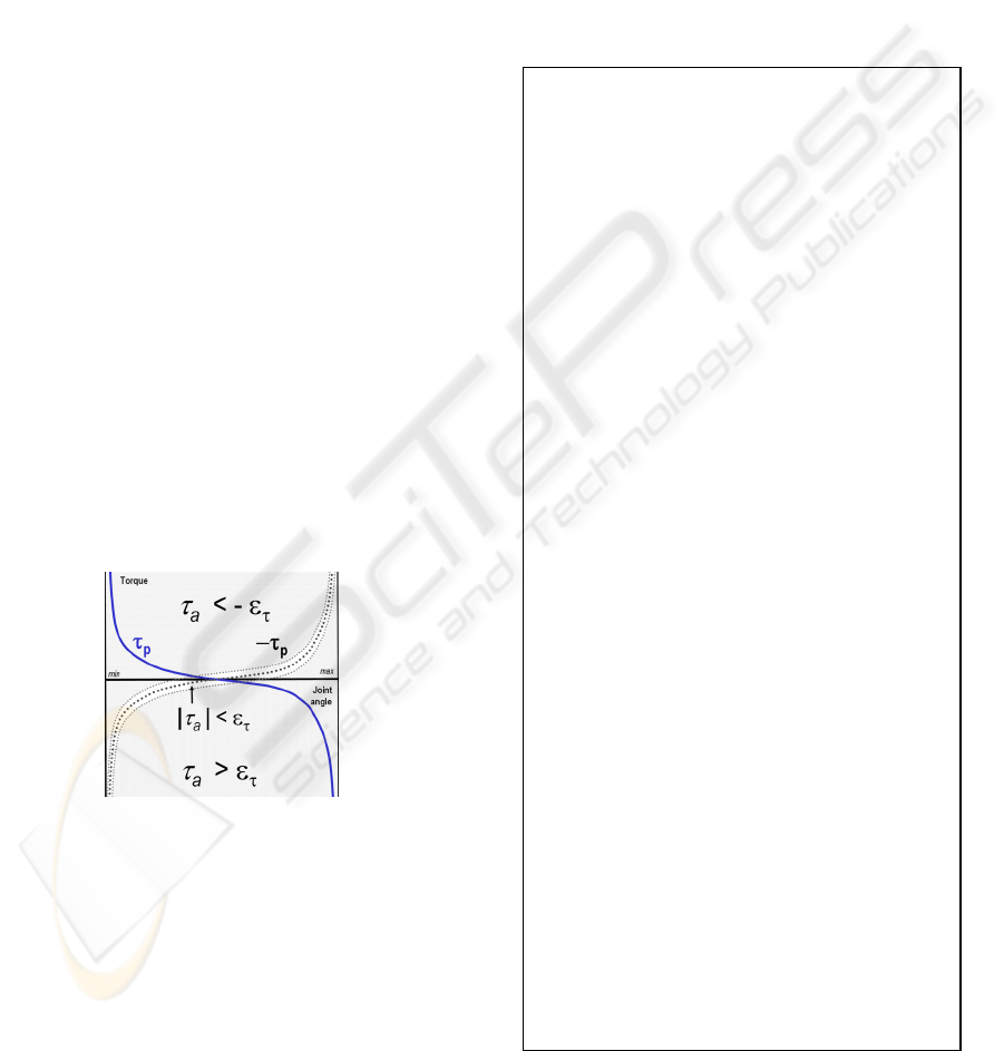
Figure 2: Sign of τ
a
with equality tolerance ε
τ.
.
The following constants or precomputed
information are useful for the algorithm too:
θ
dτ_p
(dτ
p
): given the slope of the external torque
dτ
e
, this function searches for the angle(s) where
dτ
p
=-dτ
e
.
dτ
p_min
: smallest passive torque slope (absolute value).
θ
dτ_p_min
: joint angle for which dτ
p
= dτ
p_min
.
θ
s_min,
θ
s_max
: pair of angle values on both sides of
θ
dτ_p_min
for which dτ
p
=-dτ
e
.
ε
τ
: equality tolerance for τ
e
= -τ
p
.
Two useful temporary variables are:
τ
a_min
: value of the estimated τ
a
minima.
θ
τ_a_min
: if (τ
a
>0)θ
τ_a_min
=θ
s_max
else θ
τ_a_min
=θ
s_min
.
In addition, the
Dichotomy function allows to
find the goal angle where the extrapolated external
torque line intersects with the opposite of the passive
torque function (dotted curve in Figure 2). Two
variants of searching DSS and DOS are detailed in
table2.
Table 1: Minimum active torque search.
Search slopes for θ
dτ_p
(−dτ
e
)
if no or only one slope
{ if(|τ
a
| < ε
τ
) θ
g
:= θ
c
// CASE 1.1
else if(τ
a
> ε
τ
)
θ
g
:= Dichotomy(θ
min
, θ
c
, θ
g
) // CASE 1.2
else
θ
g
:= Dichotomy(θ
c
, θ
max
, θ
g
) // CASE 1.3
}
else // two slopes
{ if(|τ
a
| < ε
τ
)
{ if( (θ
s_min
< θ
c
< θ
s_max
) or
[(θ
c
<θ
s_min
OR θ
c
>θ
s_max
)
and(sign(τ
a
(θ
s_min
)=sign(τ
a
(θ
s_max
))])
θ
g
:= θ
c
// CASE 2.1
else
{ if(active) ) // CASE 2.2
Dichotomy(θ
s_min
,θ
s_max
,θ
g
)
else θ
g
:= θ
c
// CASE 2.3
}
}else // |
τ
a
| > ε
τ
{ if( sign(τ
a
) = sign(τ
a
(θ
s_min
))
and sign(τ
a
) = sign(τ
a
(θ
s_max
)) )
{if(active AND((τ
a
-τ
a
(θ
τ_a_min
))/τ
a
> R
min
)
θ
g
:= θ
τ_a_min
// CASE 3.1
else // CASE 3.2
θ
g
:= DSS(τ
a
,θ
min
,θ
max
, θ
s_min
,θ
s_max
)
}
else
{if(active) ) // CASE 3.3
θ
g
:= Dichotomy(θ
s_min
,θ
s_max
)
else // CASE 3.4
θ
g
:= DOS(τ
a
,θ
c
,θ
min
,θ
max
, θ
s_min
,θ
s_max
)
} } }
R = (τ
a
- τ
amin
) /τ
a
(3)
SIMULATING REACTIVE/PASSIVE POSTURES BY MEANS OF A HUMAN ACTIVE TORQUE HYBRID
MINIMIZATION
7

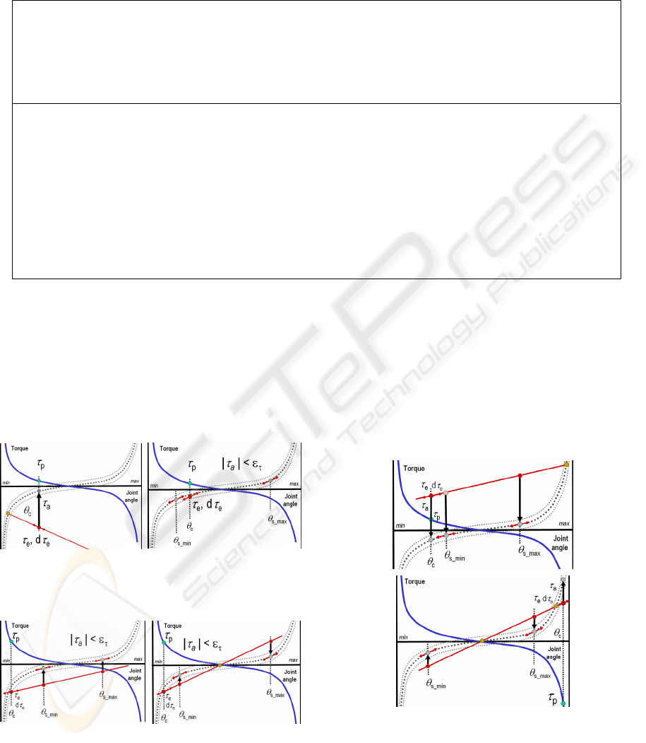
The following figures illustrate the different
cases of the hybrid minimization. Figure 3a is a case
where no active solution can be found as no slope in
the function -τ
p
matches dτ
e
. A passive solution is
found by dichotomy (intersection of the external
torque line with the opposite of the passive torque
function). In Figure 3b the current state is already
optimal.
Figure 3: (a) CASE 1.2: no slope in -τ
p
matching dτ
e
,
(b) CASE 2.1:
τ
ε
τ
<||
a
and (θ
s_min
<θ
c
<θ
s_max
).
Figure 4: (a) CASE 2.1:
τ
ε
τ
<||
a
and (θ
c
<θ
s_min
or
θ
c
>θ
s_max
)and (sign(τ
a
(θ
s_min
) = sign(τ
a
(θ
s_max
))
(b) CASE 2.2,CASE 2.3:
τ
ε
τ
<||
a
and (θ
c
<θ
s_min
or θ
c
>θ
s_max
) and (sign(τ
a
(θ
s_min
)) ! = sign(τ
a
(θ
s_max
)).
In Figure 4 the current state belongs to the
equality approximation but this time the joint angle
is smaller than θ
s_min
, hence one more sign test is
required to determine whether another joint angle,
closer to the mid-range, exists. One is found only in
Figure 4b because the active torque changes sign
between θ
s_min
and θ
s_max
, while this is not the case
for Figure 4a.
Figure 5: (a) CASE 3.1,CASE 3.2: |τ
a
| > ε
τ
and(sign(τ
a
)=sign(τ
a
(θ
s_min
))and(sign(τ
a
)=sign(τ
a
(θ
s_max
))), (b) CASE 3.3,CASE 3.4: |τ
a
| > ε
τ
and
(sign(τ
a
)!=sign(τ
a
(θ
s_min
))or
(sign(τ
a
)!=sign(τ
a
(θ
s_max
))).
Table 2: Functions defining intervals of dichotomic search (general algorithm-cases 3.2 and 3.4).
DSS(τ
a
,θ
min
,θ
max
, θ
s_min
,θ
s_max
) := Dichotomy( SameSignMinandMax(τ
a
,θ
min
,θ
max
, θ
s_min
,θ
s_max
), θ
g
)
SameSignMinandMax(input: τ
a
, θ
min
, θ
max
, θ
s_min ,
θ
s_max
,output:SameSignMin,SameSignMax) {
if(τ
a
> ε
τ
) // τ
e
is below the curve - τ
p
(θ)
{ SameSignMin := θ
min
, SameSignMax := θ
s_min
}
else //
τ
e
is above the curve - τ
p
(θ)
{ SameSignMin := θ
s_max
, SameSignMax := θ
max
}
}
DOS(τ
a
,θ
c
,θ
min
,θ
max
, θ
s_min
,θ
s_max
):= Dichotomy( OppoSignMinandMax(τ
a
,θ
c
,θ
min
,θ
max
, θ
s_min
,θ
s_max
), θ
g
)
OppoSignMinandMax (input : τ
a
, θ
c
, θ
min
, θ
max
, θ
s_min ,
θ
s_max
output:OppoSignMin,OppoSignMax){
if(τ
a
> ε
τ
) // τ
e
is below the curve - τ
p
(θ)
if( θ
c
< θ
s_max
) { OppoSignMin :=θ
min
, OppoSignMax :=θ
s_min
}
else { OppoSignMin :=θ
s_max
, OppoSignMax :=θ
max
}
}
else //
τ
e
is above the curve - τ
p
(θ)
{
if( θ
c
> θ
s_min
) { OppoSignMin :=θ
s_max
,OppoSignMax :=θ
max
}
else { OppoSignMin :=θ
min
, OppoSignMax :=θ
s_min
}
} }
a b
a
b
a b
GRAPP 2007 - International Conference on Computer Graphics Theory and Applications
8

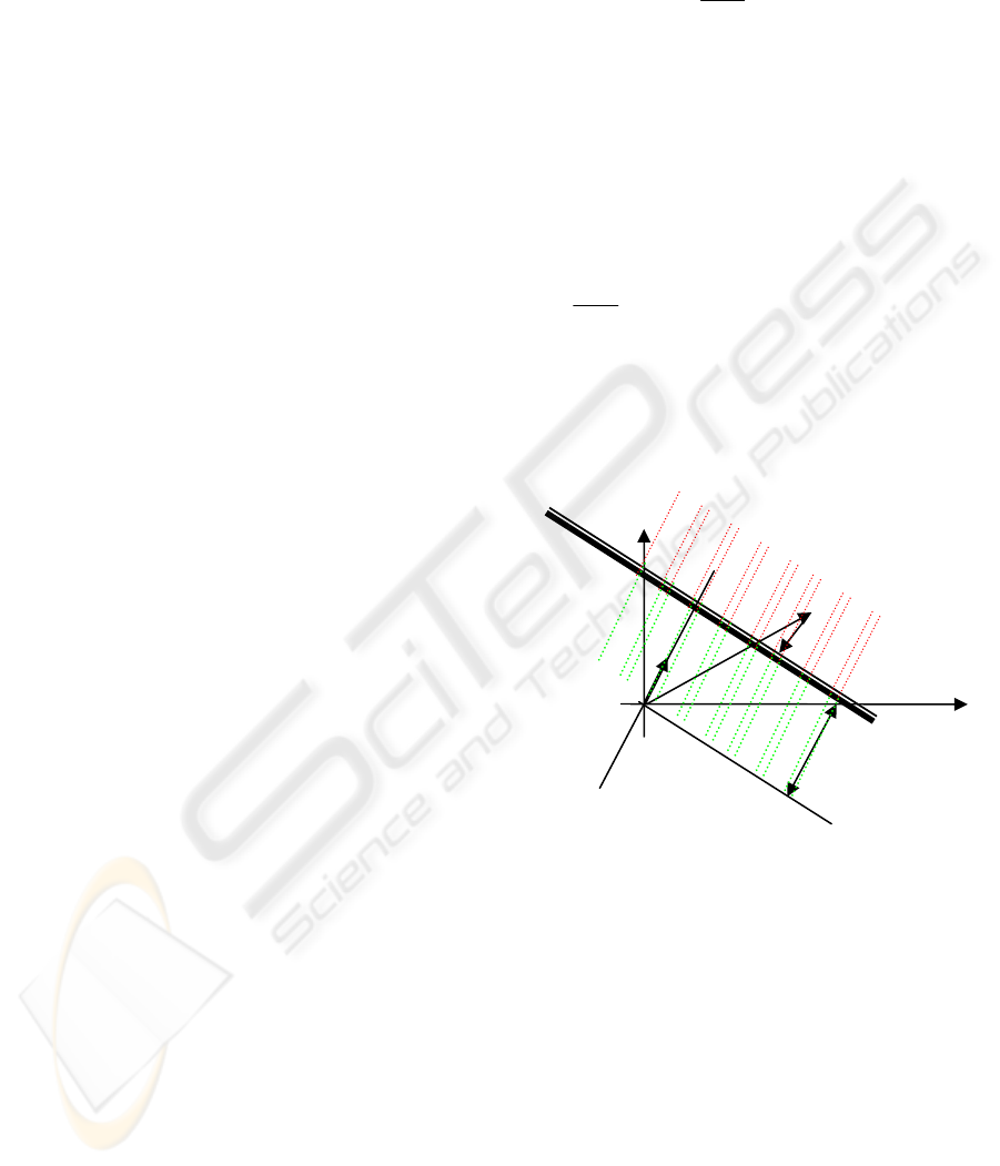
Figure 5 illustrates cases where the current active
torque is not null (e.g. a downward black arrow
indicates a negative value). In Figure 5a the two
angles θ
s_min
and θ
s_max
, with the same slope as dτ
e
indicate extrema of the active torque variation (with
constant sign), the minimum amplitude being
obtained for θ
s_min
. In Figure 5b the active torque
changes sign between θ
s_min
and θ
s_max
. If the
strategy is active a search is conducted within this
interval, otherwise the closest solution is found.
3 ALGORITHM EXPLOITATION
The reduced active torque algorithm is exploited,
within a context of posture adjustment, by means of
an Inverse Kinematics engine (Baerlocher et al.,
2004). When a muscle group reaches critical fatigue
levels (Rodríguez, 2004), the active torque reduction
algorithm proposes a target joint angle reducing the
active torque, hence the fatigue too.
In our fatigue reduction scheme we enforce a
hard linear inequality constraint whenever the active
torque amplitude of a fatigued joint i has to be
reduced:
where θ represents the n-dimensional vector of joint
coordinates, a
i
is the n-dimensional gradient vector
of the inequality constraint hyperplane and b
i
is a
scalar. Figure 6 illustrates the construction of one
inequality constraint in 2D, the current configuration
θ is out of the feasible region, requesting a ∆θ to
drive it to the feasible region. This variation vector
has an opposite direction to the constraint gradient
vector a
T
:
The scalar product of a
T
with any θ
Η
lying on
the hyperplane, such as θ + ∆θ, gives the scalar b:
We have all the elements, as shown in formula
(4), that define a fatigue reduction inequality
constraint for guiding a posture from an unfeasible
region to a feasible one.
In the following we describe how the joint
variation ∆θ has to be computed in order to adjust
the posture leading to a minimization of active
torque and therefore to a less fatigued posture.
The vector Jτ
el
gathers the partial derivatives of
its external torque τ
el
with respect to all joints:
nj
j
l
e
el
J
,1=
⎪
⎭
⎪
⎬
⎫
⎪
⎩
⎪
⎨
⎧
=
δθ
δτ
τ
(7)
Its scalar component
δτ
el
/ δ θ
l
for the fatigued joint
l is the constant external torque derivative d
τ
e
used
in the general algorithm from Table 1.
To compute Jτ
el
, we need the Jacobians J
Ti
associated with the external forces f
i
and the gravity
Jacobian J
G
associated with the weight w. This is the
expression of the partial derivative corresponding to
joint j:
).().(
__ jlG
ne
i
jilTi
j
l
e
rwJrfJ ×+×=
∑
δθ
δτ
(8)
where ne is the number of external forces, J
Ti_l
is the
column l of J
Ti
, J
G_l
is the column l of J
G
associated
with the weight w, and r
j
represents the unit axis of
rotation of joint j.
Figure 6: Example of hyperplane in 2D.
The general algorithm presented in Table 1
exploits the scalar component d
τ
e
corresponding to
δτ
el
/ δ θ
l
. It proposes a target joint angle θ
g
used to
build the component l of the posture variation
∆θ
associated to the inequality constraint bringing the
posture in the fatigue recovery region:
where θ
c
is the current joint angle, β is a positive
number smaller than 1 for stability and
∆θ
max
is a
small amplitude compatible with the small variation
hypothesis.
The fatigue reduction constraints are managed by
hysteresis thresholding which forces a minimal
i
T
i
ba <=θ
(4)
)(∆θnormalizeda
T
−=
(5)
H
θ
T
ab =
(6)
∆
θ
l
= min( β (θ
g
- θ
c
), ∆θ
max
)
(9)
θ
1
θ
2
a
b
feasible region
θ
∆θ
ba
T
=θ
ba
T
<θ
unfeasible region
ba
T
>θ
SIMULATING REACTIVE/PASSIVE POSTURES BY MEANS OF A HUMAN ACTIVE TORQUE HYBRID
MINIMIZATION
9

duration for the recovery by setting a lower
threshold for de-activating the constraints. The
process is iterated to converge toward a fatigue-
reducing posture that achieves other user-defined
tasks (e.g. reach, balance, etc…).
The fatigue reducing constraint is updated and
maintained until a recovery level is achieved. At that
point the constraint is deactivated, hence enlarging
the solution space for achieving the user-defined
tasks.
4 RESULTS
In this section we focus on three case of elbow
flexion/extension in various body postures: frontal,
oblique and lateral upper arm. In all cases, the initial
posture is due to a position task achieved by Inverse
Kinematics. This task leads to the emergence of
fatigue until a critical level that triggers the fatigue
reduction constraint (Rodríguez, 2004). We
especially examine the convergence behaviour
resulting from the iterative hybrid active torque
minimization until the active torque is effectively
reduced. This behaviour depends on the strategy
type active vs passive (see section 2.1) and the user-
given decreased ratio R
min
(see section 2.2). The
active torque (yellow curve) is iteratively minimized
from an initial posture (black point) towards a final
one where a goal with reduced active torque (green
point) is achieved.
It is important to recall that in the three studied
cases the external torque is induced by the gravity,
and the only joint that moves is the elbow. This
allows to draw the external torque function (i.e. the
red curve on Figure 1, Figure 10 and Figure 12),
however only the local knowledge of the external
torque is exploited in the following results.
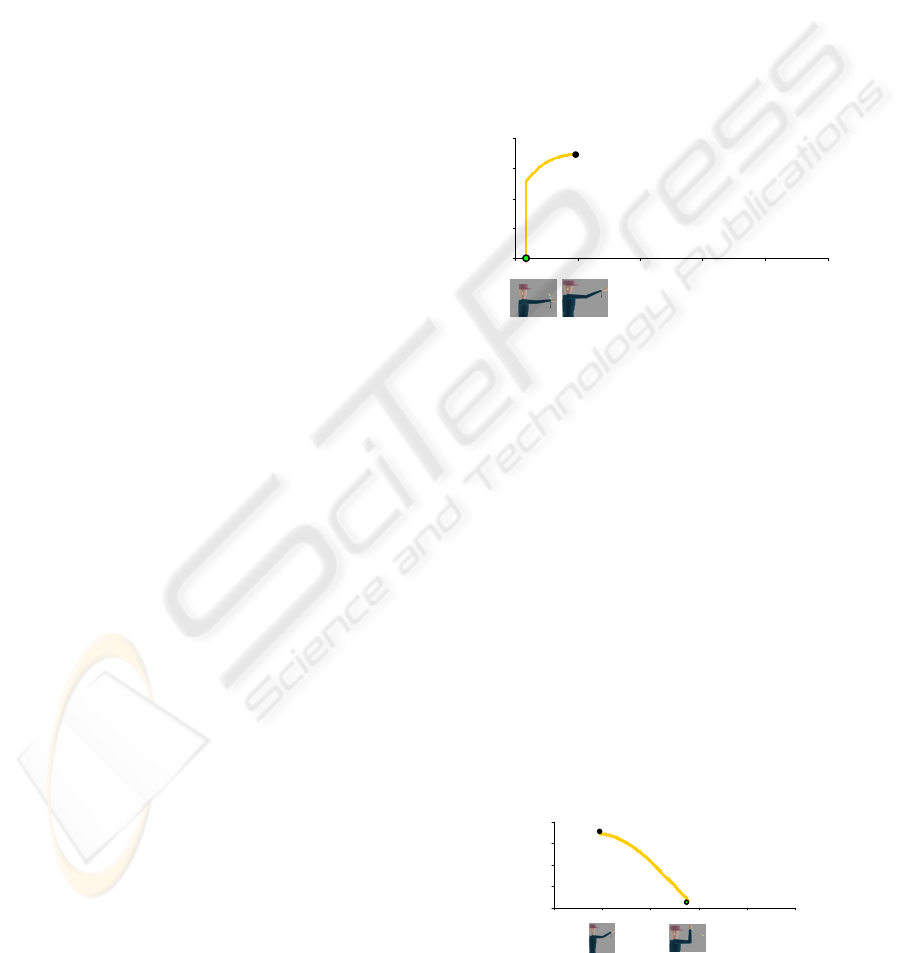
4.1 Horizontal Upper Arm
The algorithm case 3.2 is first iteratively executed in
Figure 7 for an active strategy with R
min
=1. The
resulting choice provided by the algorithm is
however a passive solution for the elbow because
the desired 100% reduction of the active torque
cannot be achieved in the mid-range of the joint
from the extrapolation of the rather flat external
torque slope (see Figure 1). As the active torque is
positive (τ
e
is below the –τ
p
(θ) curve), a dichotomic
search is done between θ
min
and θ
s_min
. After some
iterations executing case 3.2, the case 2.1 is executed
as the joint active torque is becoming smaller than ε
τ
(i.e. the current external torque is between the two
small dotted curves shown in Figure 2). As the
current state is close to the limit region and the
active torque does not change sign between θ
s_min
and θ
s_max
, the algorithm keeps the current state as
goal state (see Figure 4a). In addition, the
convergence illustrated in Figure 7 is also obtained
for a passive strategy.
In Figure 7 and Figure 9 there is a discontinuity
at the end of the convergence towards the goal; this
is due to the use of a reshaped passive torque
function. It is done via the inclusion of two linear
terms close to both joint extremes. It ensures that,
for extreme passive solutions, passive torque value
is big enough to compensate external torque.
Figure 7: (1) R
min
=1 and active strategy (2) passive
strategy. Algorithm’s cases 3.2 and 2.1 are successively
executed.
In Figure 8 the strategy is also active but the
given minimal reduction ratio,
R
min
, is much smaller
with a value of 0.2. So it is possible to find a mid-
range solution where at least a 20% of active torque
reduction is achieved. The case 3.1 is first executed,
the goal angle being defined by θ
τ_a_min
which value
for a positive active torque is θ
s_max
(i.e. τ
e
is below
the –τ
p
(θ) curve). After some iterations, the case 3.3
is executed owing to the large derivative of the
external torque (i.e. the line τ
e
(θ) crosses the –τ
p
(θ)
curve). The continuity of the provided solution is
preserved by the algorithm as the solution returned
by the dichotomic search between θ
s_min
and θ
s_max
is
close to θ
s_max
given by the previous searches.
Finally, case 2.1 is executed when τ
a
becomes
smaller than ε
τ
.
Figure 8: R
min
=0.2 and active strategy. Algorithm’s cases
3.1, 3.3 and 2.1 are successively executed.
active t o rq ue
0
1
2
3
4
0 30 60 90 120 150
elbow angle
Goal with reduced τ
a
Initial posture
acti ve tor que
0
1
2
3
4
0 306090120150
el bow a ngl e
Goal with reduced
τ
a
Initial posture
GRAPP 2007 - International Conference on Computer Graphics Theory and Applications
10

The passive strategy adopted in Figure 9 and the
active torque sign change between θ
s_min
and θ
s_max
(see Figure 5b), lead to execute case 3.4 which
returns the first passive solution in the direction of
torque active decreasing amplitude, i.e. close to the
upper limit. During the last iterations the case 2.3 is
executed when τ
a
becomes smaller than ε
τ
, which
maintains the current extremal/passive solution.
Figure 9: Passive strategy. Algorithm’s cases 3.4, and 2.3
are successively executed.
4.2 Oblique Upper Arm
Figure 11
shows the only solution obtained by
simulations for different combinations of parameters
(strategy active or passive, R
min
=1 or R
min
=0.2). Note
how it coincides with the solution given by the
particular study depicted in Figure 10.
During the first iterations, the small positive
external torque slope leads to execute the case 3.2
because the active torque does not change sign and it
is positive. Then the solution is given by dichotomic
search between θ
min
and θ
s_min
. During the last
iteration, when the active torque has been reduced
under ε
τ
, the case 1.1 is executed, returning as
solution the current angle, due to the negative values
of external torque slope and, in consequence, the
failure in the search slope (no angle where dτ
p
=-
dτ
e
).
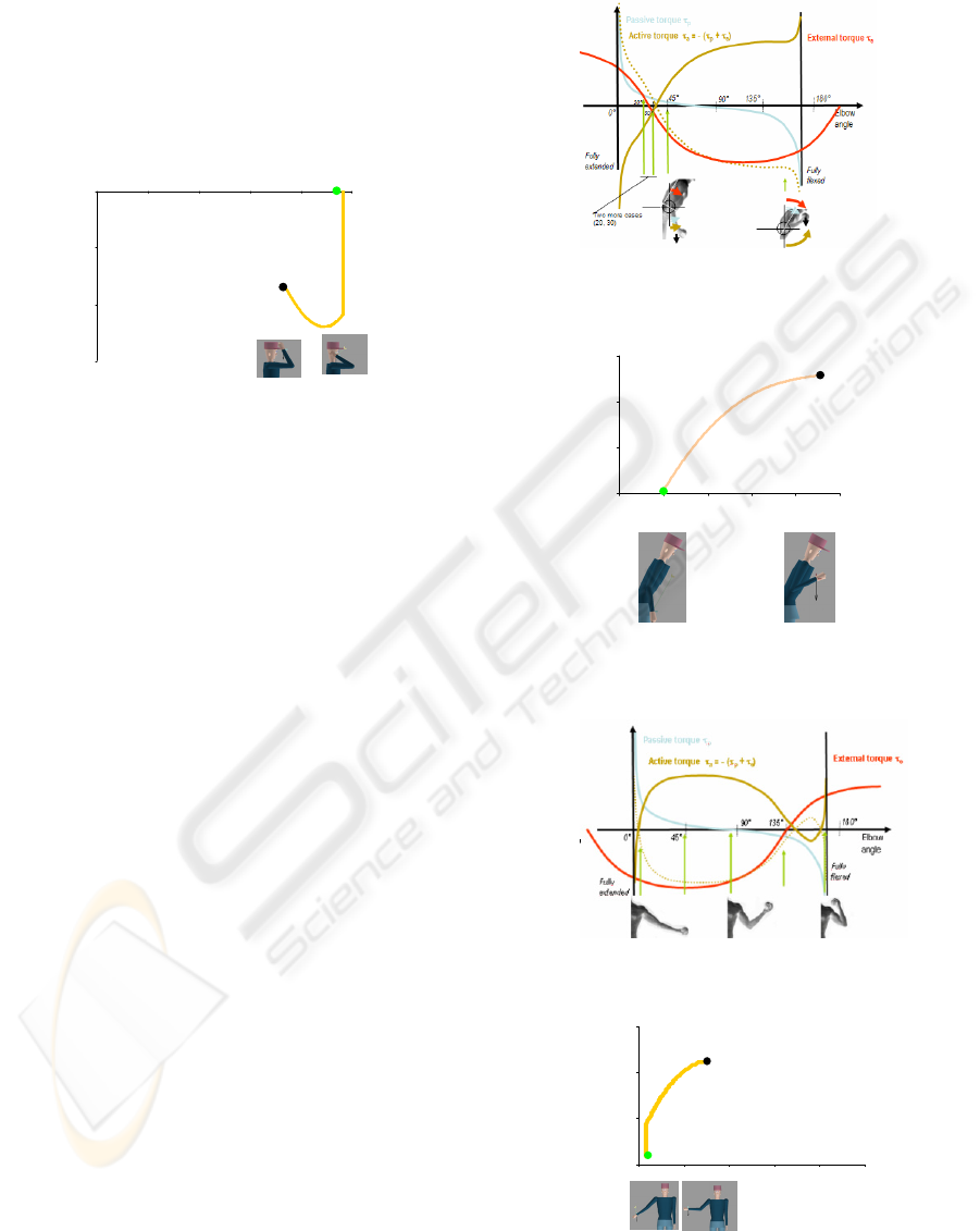
4.3 Lateral with Oblique Upper Arm
This case study is shown in Figure 12. A simulation
using Rmin=1 and active, or passive strategies (see
Figure 13), returns a passive solution as depicted in
the previously described oblique upper arm case
study (firstly case 3.2 is executed, and finally case
1.1).
Using Rmin=1 and active strategy is illustrated
on Figure 14 in the other side of the joint range. The
external torque slope is large and case 3.3 is
executed because τ
e
crosses the –τ
p
(θ) curve, then an
active solution is found when a dichotomy search
between θ
s_min
and θ
s_max
is performed. Finally, case
2.1 is executed.
Figure 10: Oblique upper arm case study.
Figure 11: R
min
=1 or 0.2 and active or passive strategies.
Algorithm’s cases 3.2 and 1.1 are successively executed.
Figure 12: Lateral with oblique upper arm case study.
Figure 13: R
min
=1 and active or passive strategies.
Algorithm’s cases 3.2 and 1.1 are successively executed.
0
2
4
6
0 30 60 90 120 150
el bow angl e
acti ve
tor que
Initial
p
osture
Goal with reduced
τ
a
0
3
6
9
0 30 60 90 120 150
elbow angle
active torque
Goal with reduced τ
a
Initial posture
3
2
1
0
0 306090120150
el bow angl e
acti ve tor que
Goal with reduced τ
a
Initial posture
SIMULATING REACTIVE/PASSIVE POSTURES BY MEANS OF A HUMAN ACTIVE TORQUE HYBRID
MINIMIZATION
11

Figure 14: R
min
=1 and active. Algorithm’s cases 3.3 and
2.1 are successively executed.
5 DISCUSSION
The main contribution of this paper is a general and
hybrid algorithm that clearly delineates all the cases
where a solution can be found in the direction
reducing the active torque amplitude (active
strategy) or in the direction of the always existing
passive solution.
The proposed technique is superior to a gradient
descent that would rely on the sole partial
derivatives of external torque and passive torque
because this latter may converge slowly or get stuck
in a local minima with null gradient.
The algorithm only makes the small assumption
that the passive-resistive torque function is a
monotonously decreasing function over the joint
range. We have introduced a user-given parameter
named the minimal active torque decrease ratio, R
min
, that leads to accept a partial decrease in the active
torque amplitude compatible with the fatigue
recovery.
The active torque reduction scheme is exploited
in a constrained Inverse Kinematics framework that
adjusts automatically fatigued postures while trying
to achieve a set of constraints representing a task
(Rodriguez, 2004). The exploited fatigue model has
been described in (Rodriguez et al., 2002).
Our future work includes the extension of the
case studies to those involving several joints. It will
allow to generate a wide range of standing poses,
including the pelvic slouch or contraposto.
In addition, we plan to take advantage of the
environment to have rest. For example, when arm
joints are too fatigued a postural change could
employ objects in the scene (e.g. a chair, a table) to
find rest.
ACKNOWLEDGEMENTS
This work has been partially supported by the Swiss
National Science Foundation.
REFERENCES
Baerlocher P., Boulic R., 2004. An Inverse Kinematic
Architecture Enforcing an Arbitrary Number of Strict
Priority Levels, The Visual Computer, Springer, 20(6)
Craig. J., 1986. Introduction to robotics : Mechanics and
control , Addison-Wesley
S. Delp, P. Loan, M. Hoy, F. Zajac, S. Fisher, J. Rosen.,
1990. An Interactive Graphics-based Model of the
Lower Extremity to Study Orthopaedic Surgical
Procedures. IEEE Transactions on Biomedical
Engineering, 37(8):757–767
Esteki A, Mansour JM, 1996. An Experimentally Based
Nonlinear Viscoelastic Model of Joint Passive
Moment. Journal of Biomechanics, 29(4):443-450
Evans P., 1979. The Postural Function of the Iliotibial
Tract. Royal College of Surgeons. 61:271-280.
Giat Y, Mizrahi J, Levy M., 1993. A Musculotendon
Model of the Fatigue Profiles of Paralyzed Quadriceps
Muscle under FES. IEEE Tran. on Biomedical
Engineering, 40(7):664–674
Hatze H., 1997. A three-dimensional multivariate model
of passive human joint torques and articular
boundaries, Clinical Biomechanics 12, 128-135
Institute ofTechnology,1998. 3, 4
Komura T, Shinagawa Y, 2001. Attaching Physiological
Effects to Motion-Captured Data. Graphics Interface
Proceedings, 27-36
Kulig K., Andrews J. G., Hay J., 1984. Human Strength
Curves. In RJ Terjung (ed) exercise sport science
reviews, 417-466. Lexington MA, DC Heath.
Kumar P., 1986. Influence of Posture on Muscle
Contraction Behaviour in Arm and Leg Ergometry.
The Ergonomic of Working Postures, ch. 16. Taylor
and Francis.
Manenica I., 1986. A Technique for Postural Load
Assessment. The ergonomics of Working Postures,
Taylor&Francis, London, 271-277
Multon F., 1988. Biomedical simulation of human arm
motion. Proceedings of the 12th European Simulation
Multiconference on Simulation - Past, Present and
Future 305 – 309. ISBN: 1-56555-148-6.
Rodríguez I, 2004. Joint level fatigue simulation for its
exploitation in human posture characterization and
optimization. PhD. Thesis, University of Alcalá.
Rodríguez I, Boulic R, Meziat D., 2002. A Joint-Level
Model of Fatigue for the Postural Control of Virtual
Humans. Human and Computer, 220-225. Tokyo
-2
-1
0
0306090120150
elbow
angle
active torque
Goal with reduced τ
a
Initial posture
GRAPP 2007 - International Conference on Computer Graphics Theory and Applications
12