
AUTOMATED COMBINED TECHNIQUE FOR SEGMENTING
CYTOLOGICAL SPECIMEN IMAGES
D. M. Murashov
Computing Centre of the Russian Academy of Sciences, 40, Vavilov street, Moscow, GSP-1, 119991, Russia
Keywords: Segmentation technique, active contour, dynamic system, height ridges, wave equation, cytological images.
Abstract: Automated snake-based combined technique for segmenting cytological images is proposed. The main fea-
tures of the technique are: implementation of the wave propagation model and modified Gaussian filter
based on the heat equation with heat source, availability of coarse and precise levels of contour approxima-
tion, automated snake initiation. The technique is successfully implemented for segmenting cytological
specimen images.
1 INTRODUCTION
One of the problems arising in the field of automated
diagnostics of hematological diseases is the segmen-
tation of nuclei in the cytological specimen images
for subsequent calculation of diagnostic features. It
is necessary to obtain such a closed curve in the
specimen image that follows the boundary of select-
ed nucleus with an adequate accuracy.
Haralick and Shapiro (Haralick and Shapiro,
1985) established the following requirements to im-
ages leading to successful segmentation: homogene-
ousness of regions in image with respect to some
characteristics; topological simplicity, significant
difference of characteristics of adjacent regions;
simplicity, smoothness, and spatial accuracy of re-
gion boundaries.
An image of a lymphoid tissue stained by Ro-
manovski-Giemsa technique is a color image (24
bpp) taken by a camera mounted on Leica DMRB
microscope using PlanApo 100/1.3 objective. The
equivalent size of a pixel was 0,0036 µ
2
. Cytological
specimen images have the following specific fea-
tures plaguing the solution. Firstly, because of poor
dye quality the boundary between cytoplasm and a
cell nucleus may be indistinctive. Secondly, cells
may be located closely to each other, in part may be
overlapped. Thirdly, adjacent nuclei may have more
strong boundaries, than selected nucleus. Fourthly,
strong edges reflecting chromatin structure inside
the nucleus appear.
Due to the features listed above any single tech-
nique failes to solve the segmentation task properly
(Bengtsson, 2004). Currently the researches more
often turn their attention to combined techniqes.
A combined technique for automated segmenting
of cell nuclei in cytological specimen images is pro-
posed. The solution of segmentation problem is ob-
tained by combining two level active contour model
and thresholding procedure with automatically esti-
mating thresold value from image histogram in CIE
Lab colour space.
Two level active contour model (or snake) is
formed using nonlinear model of a dynamic system
in terms of state-space. A snake can be initiated in
automated and manual modes. Taking into account
the properties of the stain, segmentation at a coarse
level is operating using blue colour component in
RGB space. Correction at precise level of segmenta-
tion is made using the green component. To elimi-
nate the influence of the neighboring nuclei bounda-
ries the modified Gaussian filter based on the heat
equation with a heat source is used. In order to in-
crease the capture range of the snake the wave
propagation model is implemented.
2 METHODS FOR SEGMENTING
SPECIMEN IMAGES
One of the popular segmentation techniques in cy-
tology is thresholding with automatically estimated
threshold value (Borst, 1979). The technique is com-
putationally simple but it is effective only in case
when objects and background differ in colour or
238
M. Murashov D. (2007).
AUTOMATED COMBINED TECHNIQUE FOR SEGMENTING CYTOLOGICAL SPECIMEN IMAGES.
In Proceedings of the Second International Conference on Computer Vision Theory and Applications, pages 238-245
DOI: 10.5220/0002071402380245
Copyright
c
SciTePress

gray level. In more complicated cases the segmenta-
tion consists in extraction of features per pixel and
their classification into different classes of sub-
regions. But in many cases the segmentation should
be controlled and the result should be corrected in-
teractively.
Using the simple techniques, one may run into
problems if the nuclei are clustered, the image back-
ground is inhomogeneous, and there are intensity
variations within the nuclei. By combining the
methods some of these problems can be solved. For
segmentation of cell nuclei in histological tissue
images, the method based on watersheds and dis-
tance transform (Malpica, 1997) was proposed. In
(
Bengtsson, 2004), a method for segmentation of cell
nuclei in tissue images by combining seeded water-
sheds with gradient and shape information was pre-
sented. The main disadvantage of these methods is
that one should have a tool for correcting the results
manually in complicated cases. In (Comaniciu,
2001) an approach based on nonparametric clusteri-
zation using gradient ascent mean shift procedure is
presented. The algorithm outlines clusters in Luv
space and marking their boundaries. But for obtain-
ing the suitable result the manual merging of clusters
is needed. In (Colantonio, 2006) a pixel-by-pixel
nural network classification procedure is presented.
The network is trained using clustering algorithm.
The procedure is efficient but a special tool for cor-
recting the results manually in difficult cases is
needed.
For segmentation of cell nuclei in histological
and cytological images, active contour models (pa-
rametric and geometric), or snakes, were used in
(Klemencic, 1998, Ortiz de Solorzano, 2001, Ley-
marie, 1990). Snakes provide the smooth contour
without gaps at the object boundary. Snakes were
firstly proposed in (Kass, 1987). The main idea of
parametric active contours is the following. Paramet-
ric active contour is defined as a curve
[
]
[
]
() (), (), 0,1sxsyss
ν
=∈ (here, s is a parameter),
that moves through the spatial domain of an image
minimizing the energy functional:
() () ()
()
()()
]
22
1/ 2
ext
S
EssEsds
αν βν ν
′′′
=++
⎡
⎣
∫
(1)
where
(
)
s
ν
′
and
()
s
ν
′′
(the first and the second
derivatives of
(
)
s
ν
with respect to s) characterize
the energy of internal forces, α and β are weighting
parameters that controls snake’s tension and rigidity,
ext
E – the energy of the external force. The external
force pulls the snake toward the object boundaries.
The functional (1) achieves its minimum at the
boundaries of the object. A gray-level image
(, )
I
xy
is considered as a function of spatial coordinate
variables (x, y).
ext
E is defined as:
[]
2
(, ) (, ) (, )
ext
Exy GxyIxy
σ
=−∇ ∗
(2)
where
(, )Gxy
σ
denotes the a Gaussian kernel with
standard deviation σ, ∇ denotes the gradient opera-
tor, * denotes the convolution. As σ increases, the
blurring appears and the capture range of the active
contour increases. The curve that minimizes (1, 2)
must satisfy the Euler equation. A numerical solu-
tion of the equation can be found using an iterative
procedure which is finished when the balance of
forces is achieved. The main disadvantage of the
method is the limited capture range. The effective
solution of this problem is the Gradient Vector Flow
(GVF) method, proposed in (Xu, 1998). Within this
framework, a new external force which is the solu-
tion of the generalized diffusion equation is used.
This force minimizes the new energy functional that
includes the term compensating the lack of force
farther away from the object boundaries. Such a
model increases the capture range and provides con-
vergence to boundary concavities, but it is computa-
tionally expensive. Geometric active contours
(Caselles, 1993) are based on the curve evolution
theory and level set method. This model is less com-
putationally expensive than parametric model and
makes it possible to segment more than one object in
the image. The model provides good results for im-
ages with high contrast. When the object boundary
has gaps, the contour leaks through the boundary. A
modified model, based on the relation between ac-
tive contours and the computation of geodesics in a
Riemannian space (Sapiro, 2001), eliminates leaking
at some extent. In (Yang, 2005) authors proposed a
combined snake-based approach to segmentation of
tissue images using colour gradients in Luv space.
For snake initializing a classifier is used. Classifier
is trained using sample images selected by experts.
Thus, one may conclude that: (a) the task of de-
velopment fully automated segmentation technique
is actual; (b) only combined techniques can provide
the suitable result; (c) snakes are efficient for seg-
menting cell nuclei images and can be used in auto-
mated tools (d) snakes also provide within the same
framework an instrument for manual segmentation
in difficult cases. In the next sections the problems
concerned with the development of automated com-
bined snake-based technique are considered.
AUTOMATED COMBINED TECHNIQUE FOR SEGMENTING CYTOLOGICAL SPECIMEN IMAGES
239

3 ACTIVE CONTOUR MODEL
For developing a segmentation technique it is neces-
sary to have a model of the object boundary.
3.1 Boundary Model
In literature an object boundary is defined as an ar-
rangement of local edges. Local edges are defined as
discontinuities in image luminance from one level to
another (Pratt, 2001). Various types of edge models
are known (Rohr, 2001). In (Belyaev, 1998, Eberly,
1994) edges are defind in terms of surface theory as
a ridge of the surface produced by the function of
the gray-level gradient module computed from the
image. In (Eberly, 1994) definitions of ridges are
given in terms of extremal intencity values, in terms
of principal curvature extremal values, and in terms
of level surface. In this work the following definition
of ridges is used (Eberly, 1994).
Let function
():
n
hx R R→ is of the class C
2
.
Definition. Define
()WHh
=
−
, where H(h) is
Hessian matrix, and let
i
λ
and
i
v , 1 in≤≤ be its
eigenvalues and eigenvectors. Assume that
1
...
n
λ
λ
≥≥ and 1 dn≤≤. A point x is a ridge point
of type n-d if
() 0
d
x
λ
> and x is a generalized maxi-
mum point of type n-d for h with respect to
1
[ ,..., ]
d
Vv v= .
The function
()hx has a generalized maximum of
type n-d at x if
() 0
T
Vhx∇= and (())
T
VHhxV is
negative definite (Eberly, 1994).
Since
22
1
( ) { | | ,..., | | }
T
idd
V H h V diag v v
λλ
=
and
the eigenvalues are ordered, the test for the ridge
point reduces to
() 0
T
Vhx∇= and 0
d
λ
> .
Let the gray image be described by the function
u(x)
∈
C
3
, u(x):R
2
→R
+
, x=(x,y)
T
. The coordinate
frame Oxyz is introduced; the plane Oxy is coinci-
dent with the image plain, and z=u(x,y). Let us con-
sider the function h(x):R
2
→R
+
,
22
() ()
xy
huuu=∇ = +xx ,
(3)
where
x
u
x
u
∂
=
∂
,
y
u
y
u
∂
=
∂
. In this case the ridge of
the surface h(x,y) will be a connected set of general-
ized maximum points of type 1 on the surface h(x,y),
vector v will be aligned with the surface principal
direction orthogonal to the ridge direction at this
point. For 2D images the following property follows
from the ridge definition (from the condition of 1-
maximum).
Property. At the ridge point of the surface h(x,y)
at least one principal direction is parallel to the co-
ordinate plane Oxy.
We consider an object in the image as a con-
nected set of points in some closed region
2
X
R⊂ .
We consider an edge in the image u=u(x,y) as a
projection of
(, )zhxy
=
ridge onto Oxy plane.
We consider the boundary of an object in the im-
age as a simple closed curve which includes the
edges separating the inner object regions from the
surrounding regions.
In the next section using the definitions and no-
tions given here, an active contour model will be
developed.
3.2 Active Contour Model
As the digital image includes a finite number of pix-
els, it is valid to present an active contour as a set of
n dynamic pointwise objects:
0
() ( ()), (0)
x
tfxtx x
=
=
,
(4)
where x=(x,y)
T
is the vector of spatial coordinates, t
is time. Function f(x(t))∈C
2
in the neighborhood of
the edge points x
e
should force the system (4) to
move towards x
e
and should provide stability with
respect to x
e
. As soon as we consider a set of points
modelling a continuous curve it is reasonable to say
about stability only along the normal to the contour
(or along the normal to the intensity edge).
Let us consider the function h(x,y) (3). The func-
tion z=h(x,y) defines the surface
23
VR⊂
. Further
on, we shall analyze the properties of the surface
z=h(x,y) in the neighborhood of points located at the
intensity edge.
Statement. If the function in the right-hand part of
the system (4) is constructed as
(, )
T
xy
f
hh=
, the
system (4) will be stable in the neighborhood of in-
tensity edge in the sense of the first Lyapunov
method (Lee and Markus, 1971):
[
]
() 0,Re () 0
x
e
exx
fx f x
λ
=
=
<
,
(5)
where
()
x
e
xx
fx
=
is a matrix of the linear approxi-
mation of the system (4) at x=x
e
.
Proof. The linear approximation of the system (4) in
the neighborhood of the edge point is described by
the equation:
.
.
xx xy
xy yy
hh
x
x
hh
y
y
⎛⎞
⎛⎞
⎛⎞
⎜⎟
=
⎜⎟
⎜⎟
⎜⎟
⎜⎟
⎝⎠
⎝⎠
⎝⎠
.
(6)
Here the system matrix is Hessian matrix. Let
O`x`y`z` be a coordinate frame with the origin at the
h(x,y) ridge point P which is projected to the edge
VISAPP 2007 - International Conference on Computer Vision Theory and Applications
240

point x
e
in the Oxy plane, the axis z` is aligned with
the surface normal, the axes O`x` and O`y` are
aligned with the principal directions (it is assumed,
that the couple of quadratic forms has different ei-
genvalues). We place the origin of the frame Oxyz in
P. Let axis Ox align with the principal direction
orthogonal to the ridge direction. The local surface
structure in the neighborhood of
2
PV∈ is deter-
mined by its Gaussian curvature
2222
1 2 '' '' '' ' '
() ( )/(1 )
xx yy xy x y
K
Phhhhh
λλ
== − ++,
where
12
,
λ
λ
are the eigenvalues of matrix
1
III
−
, I
and
II are matrices of the first and the second fun-
damental quadratic forms. Gaussian curvature sign is
the same as one of Hessian matrix determinant.
The following cases are considered.
1.
O`x`y` plane is tangent to (, )hxy surface and
coinsides with
Oxy. In this case
'
0
x
h = and
'
0
y
h
=
,
'' ''
0
xy yx
hh==. If P is the local maximum, then
1
0
λ
< ,
2
0
λ
< . The system (6) splits into two inde-
pendent equations. In this case, the system matrix is
the Hessian matrix, and its eigenvalues are equal to
the principal curvatures
12
,
λ
λ
of (, )hxy at the
point P. Hence, the system is stable according to the
first Lyapunov method.
2. O`x`y` plane is tangent to
(, )hxy surface and
coinsides with Oxy plane,
'' ''
0
xy yx
hh==
,
1''
x
x
h
λ
=
,
2''yy
h
λ
= . The O`x`y` plane is tangent to the surface
and parallel to the Oxy plane. In this case
'
0
x
h
=
and
'
0
y
h = . Let us assume
1
0
λ
< ,
2
0
λ
= (or
1
0
λ
=
,
2
0
λ
< ). Then the system will be stable in the sense
of the first Lyapunov method along the Ox axis and
neutral along the Oy axis. So, an object (4) will
move from some initial point (x
0
,y
0
) to a point (0,y
0
).
3. O`x`y` plane is tangent to
(, )hxy surface and
coinsides with Oxy plane,
'
0
xx
hh==, and
'
0
yy
hh==
;
1
0
λ
< ,
2
0
λ
> , or vise versa. In this
case, P is a saddle point, and the system is stable
along one of the principal directions and tends to the
closest local maximum along another one. So, at the
steady state the pointwise objects move permanently
along the curvature lines from the
(, )hxy saddle
points towards the nearest local maxima or parabolic
points. Hence, the snake is stable with respect to the
intensity edge.
4. O`x`y` plane is tangent to
(, )hxy surface but
does not coinside with Oxy (see Figure 1). Accord-
ing to the property of ridge points, at least one of the
prncipal directions is parallel to image plane. Let
axis O`x` be in Oxy plane. Axis O`x coinsides with
Ox` and Oy axis directed along the projection of
O`y` axis onto Oxy plane. In O`x`y`z` frame the sur-
face will be described by a function
'(',')zxy
ϕ
=
.
(7)
We shall find out how the Hessian matrix and its
eigenvalues will change in Oxyz frame. Coordinates
x`, y`, z` are transformed to coordinates x, y, z ac-
cording to the following expression:
22
10 0
'
0cos sin ,
0sincos
'
'
xx
y
z
y
z
π
π
θ
θθ
θθ
<<=−
−
⎛⎞
⎡⎤ ⎡ ⎤
⎜⎟
⎢⎥ ⎢ ⎥
⎜⎟
⎢⎥ ⎢ ⎥
⎜⎟
⎢⎥ ⎢ ⎥
⎣⎦ ⎣ ⎦
⎝⎠
.
Taking into account that
'
0
x
ϕ
= and
'
0
y
ϕ
= it is
shown that the elemets of the Hessian matrix will be
as follows:
2
''
2
cos
x
x
z
x
ϕ
θ
∂
=
∂
,
2
0
z
xy
∂
=
∂∂
,
2
''
23
cos
yy
z
y
ϕ
θ
∂
=
∂
.
(8)
Figure 1: The surface z=h(x,y) and coordinate frames.
From (8) follows that theHessian is the diagonal
matrix and the signs of the eigenvalues depend on
cosθ sign. The expressions (8) can be justified by
comparing formulas for Gaussian and mean curva-
ture in both coordinate frames. Hence, as in cases
described above, the linear approximation of the
system (4) splits into two independent equations
with respect to variables x and y. According to the
conditions (5) the sysytem (4) will be stable with
rspect to intensity edge. The statement is proofed.
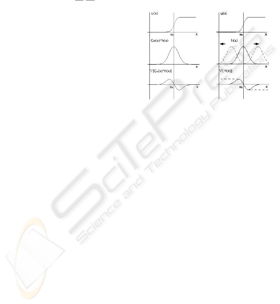
In practice, the function in the right-hand part of
the system (4) may be composed of several compo-
nents. The main component f
0
is formed as a
smoothed image edge map:
0
() [ () ()]
f
xGxhx
σ
=∇ ∗ ,
where x=(x,y)
T
, G is the Gaussian kernel with stan-
dard deviation σ,
∇
is the gradient operator. The
appearance of f
0
(x) for 1-D case and the stages of
forming are shown in Figure 2 (a). Also, a smooth-
ing term of the form
11 max
()/| |kf x f (here
1
()
f
x char-
AUTOMATED COMBINED TECHNIQUE FOR SEGMENTING CYTOLOGICAL SPECIMEN IMAGES
241
acterizing the curvature, f
max
is the maximum value
of f
0
(x)) is introduced in (4). Let
()
() (), ()
T
Cs xs ys=
be a parameterized representation of the contour at
fixed instant of time t, here, s - is the Euclidian arc
length. We define
1
()
f
x by the expression:
1
() ()
ss
f
xCs= ,
22
22
,()
T
ss
dx dy
ds ds
Cs
⎛⎞
=
⎜⎟
⎝⎠
.
Thus, the equation describing the dynamics of the
pointwise object will be as follows:
(
)
0max11max
()/| | ()/| |
x
t fxf kfxf=+
,
(9)
Coefficient k
1
is calculated from the stability condi-
tions of model (9). To eliminate discontinuities and
redundant contour points during evolution, resam-
pling procedure is applied. For segmenting images
with low contrast boundaries of the objects of inter-
est and high contrast boundaries of adjacent objects,
the two-level algorithm is proposed. At the first
level, the coarse approximation of the boundaries is
obtained. At the second level, the contour evolution
results in precise boundary approximation.The initial
condition of model (9) at the first level is the given
initial contour, for example, an elipse. Initial condi-
tion at the second level is the contour obtained at the
first level. The accuracy of segmentation substan-
tially depends on nucleus edge map quality. At the
first level, where the main goal of preprocessing is
the obtaining of coarse nucleus edge map and sup-
pression of high contrast edges of adjacent nuclei,
the blue component of the input image is used. At
the second level, where contour evolution results in
precise boundary approximation, the influence of
adjacent nuclei is not crucial, but it is necessary to
operate with more precise and strong nucleus edge
map. In this case, color reduction is performed by
subtracting the green component from the input im-
age.
3.3 Expanding the Capture Range
Within the developed technique, thresholding and
subsequent Gaussian blurring are applied to the
function h(x,y) in order to strengthen and to level off
the edge map. The standard deviation σ determines
the capture range of the model (4). At large σ, the
boundaries of the objects in the analyzed image dis-
appear and the adjacent objects merge. The pre-
sented model accurately segments the objects of
simple shapes with smooth boundaries. But it fails to
segment the images with boundary concavities. Xu
and Prince (Xu and Prince, 1998) proposed the GVF
model that uses the vector field to force the snake to
move. The vector field is computed from the image
as the steady-state solution of a pair of linear partial
differential equations. The GVF model provides the
ability to move the snake into boundary concavities
but it is computationally expensive. In this paper, in
order to expand the capture range of the model (4),
the model of wave propagation is used. The main
idea is to spread the large values of the function in
the right-hand part of (4) (see Figure 2 (b)).
(a)
(b)
Figure 2: Constructing active contour model: (a) forming
component f
0
(x) for 1-D case, top – object boundary, mid-
dle – smoothed edge map, bottom – function f
0
(x); (b)
expanding the capture range of the active contour model.
Unlike the GVF model, there is no need to obtain
the steady-state solution of differential equations.
For this model, the Cauchy problem for the hyper-
bolic partial differential equation is solved with the
initial conditions w=
(, )Ghxy
σ
, w
t
=0:
2
2222
0
(, ,) ( , ,),
() (,), / / ,
tt
wxyt a wxyt
wt Ghx y x y
σ
=Δ
=
Δ=∂ ∂ +∂ ∂
(10)
where
G
σ
is the Gaussian kernel with standard de-
viation σ. Equation (10) describes the wave propa-
gation process generated by the smoothed edge map.
When solving equation (10) at each instant of time t
at a point (x,y) the values of
,
x
y
ww are calculated,
and maximal absolute values at the wave front are
stored. The sign of the stored value is the same as
the sign of the first nonzero value of
,
x
y
ww calcu-
lated at this point. Thus, the maximal gradient values
of the function
(, )Ghxy
σ
propagate inside and out-
side the object boundary in natural way. The size of
this region is defined by the value of at. In result, the
vector field that forms the right hand part of model
(4) is obtained. In Figure 3 (a)-(e) an example of
segmenting of an object with non-convex boundary
is shown: (a) – initial contour approximation, (b) –
smoothed edge map, (c) and (d) -
,
x
y
ww
, (e) – re-
VISAPP 2007 - International Conference on Computer Vision Theory and Applications
242
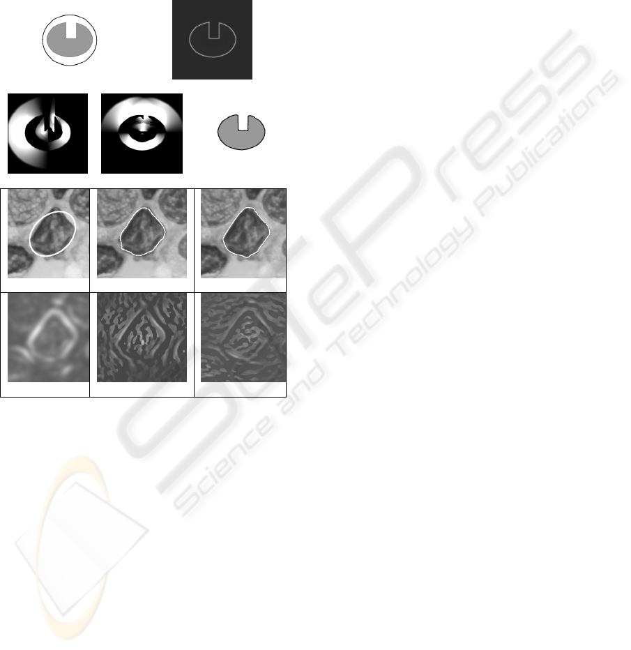
sulting contour, bright regions correspond to positive
values, dark ones – to non-positive values. The
frame origin is at the top left corner of the image. In
Figure 3 (f)-(k) the results of cell nucleus segmenta-
tion are shown: (f) – the initial contour approxima-
tion; (g) – coarse approximation; (h) – precise ap-
proximation, (i) – blurred edge map
(, )Ghxy
σ
; (j),
(k) –
,
x
y
ww at the second level.
(a)
(b)
(c)
(d)
(e)
(f)
(g) (h)
(i)
(j)
(k)
Figure 3: Image segmentation process: (a) – (e) – artificial
image, (f) - (k) – cytological image.
3.4 Modified Gaussian Filter
For the successful operating of the active contour
model two problems should be solved. Firstly,
strong edges at the boundaries of the segmented nu-
cleus should be obtained. Secondly, strong edges at
the boundaries of the adjacent nuclei should be sup-
pressed. For constructing function f
0
(x) in the right-
hand part of the active contour model (9) Gaussian
blur is used for image smoothing before obtaining
the edge map h(x) and then for blurring h(x).
For suppressing strong edges at the boundaries of
adjacent nucleus the modified Gaussian filter was
applied. The Gaussian kernel used in a standard
Gaussian filter is the fundamental solution of a heat
equation (Koederink, J., 1984). The modified filter is
constructed on the basis of a heat equation which
features the development of two-dimensional non-
stationary process in the fixed environment with heat
sources or sinks:
(, ,),
txxyy
uu u Fxyt−=+
00
() ,ut u=
0 f
ttt≤≤ ,
(11)
here,
(, ,)uuxyt
=
is the image under processing,
,
x
y - are the spatial coordinates, t is time, t
0
, t
f
are
initial and final moments. On the one hand, for im-
age smoothing before obtaining edge map, the func-
tion
(, ,)
F
xyt describing a source or sink of heat,
should be designed so that the adjacent nuclei should
not be smoothed and merge with one of interest. On
the other hand, the function
(, ,)
F
xyt should not
generate the strong
edges in the image edge map.
Thus, we may define this function as follows:
0
0
,( , ) int( );
(, ,)
0, ( , ) int( ),
xx yy
uuxy C
Fxyt
xy C
+∉
⎧
⎪
=
⎨
∈
⎪
⎩
(12)
where
0
int( )C denotes the set of points (, )
x
y inside
the initial approximation of contour
0
C .For blurring
the edge map the function
(, ,)
F
xyt should be cre-
ated so that it should essentially reduce the intensity
of the pixels outside the initial contour
0
C . For ex-
ample, the function may be defined as follows:
0
(, ,) *C[ [ ( )]]
B
Fxyt G FILL C
σ
δ
= ,
(13)
for
0 f
ttt
≤
≤ , where
0
C denotes the initial contour,
B
δ
denotes the dilation operator with the structuring
element B, FILL denotes the fillhole operator (Soille,
2004),
G
σ
is the Gaussian kernel with standard de-
viation σ, * denotes the convolution, and
C denotes
the complementation operator. The size of structur-
ing element B is set equal to σ. The initial approxi-
mation of the contour in this case should be set out-
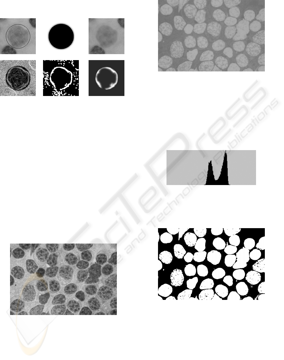
side of the selected nucleus. In Figure 5 the stages of
constructing the function f
0
(x) in the right-hand part
of model (9) using the modified Gaussian filter with
different functions
0
(, , )
F
xyt are illustrated. In Fig-
ure 4 (a) the given fragment of the preparation image
with the initial contour
0
C is shown. In Figure 4 (b)
0
(, , )
F
xyt is shown. Figure 4 (c) the result of the
initial image blurring with function
0
(, , )
F
xyt de-
fined by (12) is presented. In Figure 4 (d) one can
see the edge map obtained from the image in Figure
4 (c). In Figure 4 (e) the result of applying morpho-
logical opening and thresholding operations to the
image in Figure 4 (d) is shown. In Figure 4 (f) the
blurred image Figure 4 (e) is presented, here the
function
0
(, , )
F
xyt is defined by expression (13).
The scheme for the numerical solution of the equa-
AUTOMATED COMBINED TECHNIQUE FOR SEGMENTING CYTOLOGICAL SPECIMEN IMAGES
243
tion (11) is based on the scheme presented in (Lin-
deberg, 1994).
(a) (b) (c)
(d) (e) (f)
Figure 4: The stages of constructing the function
f
0
(x)
using modified Gaussian filter: (a) the given fragment of
the preparation image and initial contour
0
C ; (b) the heat
source function
0
(, , )
F
xyt ; (c) blurred image (a), the
function
0
(, , )
F
xyt is defined as (12); (d) the edge map
obtained from image (c); (e) the result of applying mor-
phological opening and thresholding operations to image
(d); (f) blurred image (e), the function
0
(, , )
F
xyt is de-
fined as (13).
4 AUTOMATED SNAKE
INITIALIZATION
In cytological specimen image segmentation tasks a
lot of objects appeared in the image (see Figure 5)
should be segmented.
Figure 5: Cytological specimen image.
The manual snake initialization making segmenta-
tion task crucially time consuming. In (Yang, 2005)
a classifier trained by example provided by experts
is applied for obtaining rough approximation of ob-
jects used for initializing GVF snake. Taking into
account instability of staining properties and condi-
tions of specimen image aquizition the experts
should train the classifier regularly.
Figure 6: Component a of the specimen image in the CIE
Lab color space.
In this work a simple automated initialization
procedure based on the specimen staining properties
is proposed. The procedure is based on the proper-
ties of specimens stained by Romanovsky-Giemza
technique. Specimen image component a in the CIE
Lab colour space (see Figure 6) has bimodal inten-
sity histogram (see Figure 7).
Figure 7: Histogram of the image shown in Figure 6.
Using thresholding operation with automatic es-
timated threshold value one can obtain a binary
mask of the specimen image (see Figure 8).
Figure 8: Binary mask of the image shown in Figure 7.
Further on, the following operations should be ap-
plied to each of the objects taken one-by-one in the
binary mask image to obtain the corresponding ini-
tial approximation of the contour. First, morphologi-
cal fillhole operation. Second, filtering by area
value. Small objects are excluded. If the object area
is large, an iterative procedure is applied to compo-
nent a image fragment in order to find the threshold
value at which the binary object splits into parts.
After that, filtering is applied to each part of the ini-
VISAPP 2007 - International Conference on Computer Vision Theory and Applications
244

tial object. Third, the white top-hat operation is ap-
plied to obtain contour initial approximation.
It is necessary to note, that at step 2 one may use
distance transform operation to separate two touch-
ing objects instead of described iterative procedure.
The iterative procedure is effective because of
smoothness of intensity histogram.
5 CONCLUSIONS
The combined technique for automated segmenting
of cell nuclei in cytological specimen images is pro-
posed. The solution of segmentation problem is ob-
tained by combining two level active contour model
and thresholding procedure with automatically esti-
mating threshold value from image histogram in CIE
Lab colour space. The main features of the technique
are: implementation of the wave propagation model
and modified Gaussian filter based on the heat equa-
tion with heat source, availability of coarse and pre-
cise levels of contour approximation, automated
snake initiation. The technique is successfully im-
plemented for segmenting cytological specimen im-
ages.
ACKNOWLEDGEMENTS
This work is partially supported by Russian Founda-
tion for Basic Research Grants NN 05-07-08000, 06-
01-81009, 06-07-89203, by the project within the
Program of the Presidium of the Russian Academy
of Sciences "Fundamental Problems of Computer
Science and Information Technologies", and by
INTAS Grant N 04-77-7067.
REFERENCES
Borst, H., Abmayr, W., and Gais, P., 1979. A thresholding
method for automatic cell image segmentation
, J. His-
tochem. Cytochem.,27
(1), pp 180–187.
Belyaev, A.G., Pasko, A.A., KuniiT.L., 1998. Ridges and
Ravines on Implicit Surfaces.
Computer Graphics In-
ternational (CGI '98), June 22-24,
Hannover, Ger-
many, pp. 530-535.
Bengtsson, E., Wahlby, C., Lindblad, J., 2004. Robust Sell
Image Segmentation Methods.
Pattern Recognition
and Image Analysis. Advances in Mathematical The-
ory and Applications. Vol.14, No. 2,
pp. 157 – 167.
Caselles, V., Catte, F., Coll, T., Dibos, F. 1993. A geomet-
ric model for active contours.
Numerische Mathematik
66
, pp. 1-31.
Comaniciu, D., Meer, P., 2001. Cell Image Segmentation
for Diagnostic Pathology,
Advanced Algorithmic Ap-
proaches to Medical Image Segmentation: State-Of-
The-Art Applications in Cardiology, Neurology,
Mammography and Pathology
. J. Suri, S. Singh and
K. Setarehdan (Eds.), Springer, pp. 541-558.
Colantonio S., Gurevich I.B. Salvetti O., 2006. Automatic
Fuzzy-Neural Based Segmentation of Microscopic
Cell Images,
In Workshop Proceedings: Petra Perner
(Ed.), Workshop on Mass-Data Analysis of Images
and Signals,
MDA 2006 IBaI CD-Report, p. 34-45.
Eberly, D., Gardner, R., Morse, B., Pizer, S., and Schar-
lach, C., 1994. Ridges for image analysis,
Journal of
Mathematical Imaging and Vision, 4, 4, December,
pp. 353 – 373
.
Haralick, R. M., Shapiro, L. G., 1985. Image Segmenta-
tion Techniques,
Computer Vision, Graphics, and Im-
age Processing, 29, 1
, pp. 100-132.
Kass, M., Witkin, A., Terzopoulos, D. 1987. Snakes: Ac-
tive contour models.
Int. Journal on Computer Vision,
1,
pp. 321-331.
Koederink, J., 1984. The structure of images.
Bio. Cy-
bern., 50,
pp.363 - 370.
Klemencic, A., Kovacic, S., Pernus, F., 1998. Automated
segmentation of muscul fiber images using active con-
tour models
, Cytometry 32, pp. 317-326.
Soille, P., 2004.
Morphological Image Analysis: Princi-
ples and Applications,
Springer-Verlag, Berlin.
Lindeberg, T., 1994.
Scale-space Theory in Computer
Vision.
Kluwer Academic Publishers.
Lee, E.B., Markus, L., 1971.
Foundations of optimal con-
trol theory,
J. Willey & Sons, Inc., New York, Lon-
don, Sydney.
Leymarie, F., 1990. Tracking and Describing Deformable
Objects Using Active Contour Models.
Technical Re-
port CIM-90-9,
McGill Research Center for Intelligent
Machines, 186 p.
Malpica, N., Ortiz de Solorzano, C., Vaquero, J.J., et. al.,
1997. Applying watershed algorithms to the segmenta-
tion of clustered nuclei.
Cytometry. 28, pp. 289-297.
Ortiz de Solorzano, C., Malladi, R., Lelievre, S.A.,
Lockett,S.J., 2001. Segmentation of nuclei and cells
using membrane related protein markers. Journal of
Microscopy, 201
, pp. 404-415.
Rohr, K., 2001.
Landmark-Based Image Analysis Using
Geometric and Intensity Models
, Kluwer Academic
Publishers, 303 p.
Pratt, W.K. 2001.
Digital Image Processing: PIKS Inside,
John Wiley & Sons, Inc., 735 p.
Sapiro, G., 2001.
Geometric Partial Differential Equations
and Image Analysis
.Cambridge University Press,
Cambridge.
Xu, C., Prince, J.L., 1998. Snakes, Shapes, and Gradient
Vector Flow.
IEEE Transactions On Image Process-
ing,
7 (3), pp.359-369.
Yang, L. Meer, P., Foran, D., 2005. Unsupervised seg-
mentation based on robust estimation and color active
contour models,
IEEE Trans. on Information Technol-
ogy in Biomedicine
, 9, pp. 475-486.
AUTOMATED COMBINED TECHNIQUE FOR SEGMENTING CYTOLOGICAL SPECIMEN IMAGES
245
