LOW COST SENSING FOR AUTONOMOUS CAR DRIVING IN
HIGHWAYS
Andr
´
e Gonc¸alves, Andr
´
e Godinho
Instituto Superior T
´
ecnico, Institute for Systems and Robotics, Lisbon, Portugal
Jo
˜
ao Sequeira
Instituto Superior T
´
ecnico, Institute for Systems and Robotics, Lisbon, Portugal
Keywords:
Autonomous car driving, Car-like robot, Behavior-based robot control, Occupancy grid.
Abstract:
This paper presents a viability study on autonomous car driving in highways using low cost sensors for envi-
ronment perception.
The solution is based on a simple behaviour-based architecture implementing the standard perception-to-action
scheme. The perception of the surrounding environment is obtained through the construction of an occupancy
grid based on the processing of data from a single video camera and a small number of ultrasound sensors.
A finite automaton integrates a set of primitive behaviours defined after the typical human highway driving
behaviors.
The system was successfully tested in both simulations and in a laboratory environment using a mobile robot
to emulate the car-like vehicle. The robot was able to navigate in an autonomous and safe manner, performing
trajectories similar to the ones carried out by human drivers. The paper includes results on the perception
obtained in a real highway that support the claim that low cost sensing can be effective in this problem.
1 INTRODUCTION
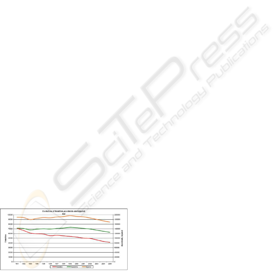
Over the last decade there has been a steady decrease
in the number of casualties resulting from automobile
accidents in the European Union roads. Still, more
than 40000 people die each year (see Figure 1) and
hence additional efforts in autonomous car driving are
socially relevant.
Figure 1: Eurostat data of sinistrality (source (EUROSTAT,
2006)).
Research on autonomous car driving systems
shows that such systems may reduce drivers stress and
fatigue resulting in a significant decrease in the num-
ber of accidents and fatalities.
Two main strategies are possible in the develop-
ment of autonomous driving systems, one acting on
the infrastructures, i.e., the highways, and the other
on vehicles. The latter has been the one which has
gathered higher acceptance throughout the scientific
community. Developing a system that has the abil-
ity to navigate in the existing road network requires
the capability of perceiving the surrounding environ-
ment. This paper describes an architecture for au-
tonomous driving in highways based on low cost sen-
sors, namely standard video cameras and ultrasound
sensors.
Nowadays, the most advanced autonomous driv-
ing systems, such as the ones which took part in the
Darpa Grand Challenge 2006, (Thrun et al., 2006;
Whittaker, 2005) embody a large number of sen-
sors with powerful sensing abilities. Despite proving
capable of autonomous navigation even in unstruc-
tured environments such as deserts, these systems are
unattractive from a commercial perspective.
A number of autonomous driving systems de-
370
Gonçalves A., Godinho A. and Sequeira J. (2007).
LOW COST SENSING FOR AUTONOMOUS CAR DRIVING IN HIGHWAYS.
In Proceedings of the Fourth International Conference on Informatics in Control, Automation and Robotics, pages 370-377
DOI: 10.5220/0001652803700377
Copyright
c
SciTePress
signed specifically for highway navigation have been
described in the literature. As highways are a more
structured and less dynamic environment, solutions
can be developed with lower production and oper-
ational costs. At an academic level, (Dickmanns,
1999) developed systems that drove autonomously
in the German Autobahn since 1985, culminating
with a 1758Km trip between Munich and Denmark
(95% of distance in autonomous driving). In 1995,
Navlab 5 drove 2849 miles (98% of distance in au-
tonomous driving) across the United States, (Jochen
et al., 1995). In 1996, ARGO, (Broggi et al., 1999)
drove 2000Km (94% of distance in autonomous driv-
ing) in Italy. At a commercial level, only recently
have autonomous driving systems been introduced.
Honda Accord ADAS (at a cost of USD 46.500), for
example, is equipped with a radar and a camera, be-
ing capable of adapting the speed of the car to traffic
conditions and keeping it in the center of the lane.
The system described in this paper, named HANS,
is able to perform several tasks in the car driving do-
main, namely, following the road, keeping the car
in the right lane, maintaining safe distances between
vehicles, performing overtaking maneuvers when re-
quired, and avoiding obstacles. Without loosing gen-
erality, it is assumed that there are no cars driving
faster than the HANS vehicle, meaning that no cars
will appear from behind.
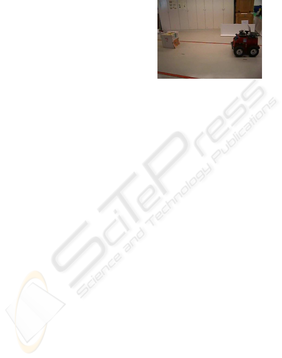
HANS uses a low resolution web camera located
in the centre of the vehicle behind the rear-view mir-
ror and a set of sixteen sonars. The camera’s objective
is to detect the road lanes and vehicles or objects that
drive ahead. The sonar is used to detect distances to
the vehicles/objects in the surroundings. HANS vehi-
cle is an ATRV robot with a unicycle-like kinematic
structure. A straightforward kinematics transforma-
tion is used such that the vehicle is controlled as if
it has a car-like kinematics. Figure 2 shows the ve-
hicle and the location of the sensors considered (the
small spheric device in the front part of the robot is
the webcam; other sensors shown are not used in this
work) The experiments were conducted in a labora-
tory environment (in Figure 2) consisting on a section
of a highway scaled down to reasonable laboratory di-
mensions. The total length is around 18 meters.
A behaviour-based architecture was used to model
the human reactions when driving a vehicle. It is di-
vided in three main blocks, common to a standard
robot control architecture. The first, named Percep-
tion, generates the environment description. It is
responsible for the sensor data acquisition and pro-
cessing. An occupancy grid (see for instance (Elfes,
1989)) is used to represent the free space around the
robot. The second block, named Behavior, is respon-
Figure 2: The HANS vehicle (ATRV robot) in the test envi-
ronment; note the obstacle ahead in the “road”.
sible for mapping perception into actuation. A finite
automaton is used to choose from a set of different
primitive behaviors defined after the a priori knowl-
edge on typical human driving behaviors. The third
block, Actuation, is responsible for sending the com-
mands to the actuators of the robot.
This paper is organized as follows. Sections 2
to 4 describe the perpection, behavioral and actua-
tion blocks. Section 5 presents the experimental re-
sults. Section 6 summarizes the conclusions drawn
from this project and points to future developments.
2 PERCEPTION
This section describes the sensor data acquisition and
processing, together with the data fusion strategy. The
environment representation method and the data fu-
sion scheme were chosen to, in some sense, mimic
those used by humans when driving a car.
2.1 Ultrasound Sensors
The space covered by the set of sonars is discretized
into an occupancy grid, where the obstacles and free
space around the robot are represented. Basic obsta-
cle avoidance is achieved by computing the biggest
convex polygon of free space in the area in front of
the robot and controlling it such that it stays in this
area.
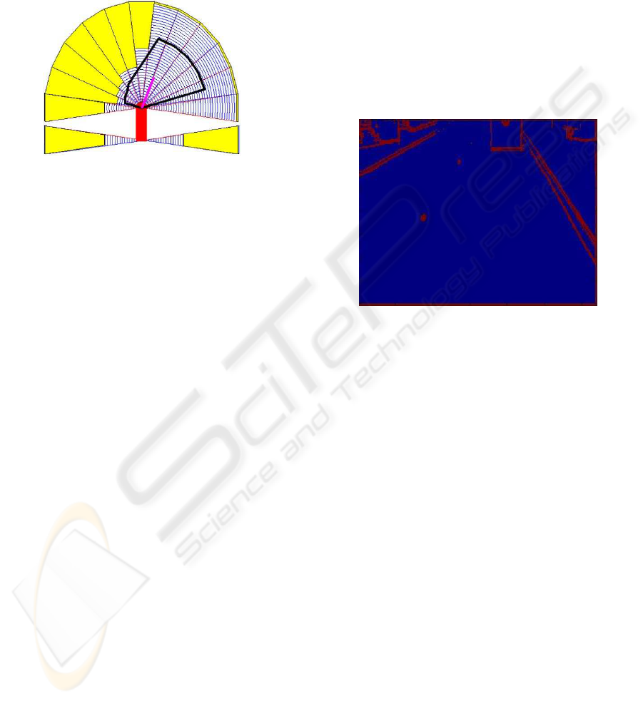
The chosen occupancy grid, shown in Figure 3,
divides each sonar cone into a number of zones, i.e.,
circular sectors, each being defined by its distance to
the centre of the robot. Each raw measurement from a
sonar is quantized to determine the zone of the grid it
belongs to. Each zone, or cell, in the occupancy grid
keeps record of the number of measurements that fell
in it. The grid is updated by increasing the value in
LOW COST SENSING FOR AUTONOMOUS CAR DRIVING IN HIGHWAYS
371
the cell where a measurement occured and decreas-
ing the cell where the previous measurement occured.
The zone with the highest number of measurements
(votes in a sense) is considered as being occupied by
an obstacle. This strategy has a filtering effect that
reduces the influence of sonar reflexions.
Figure 3: Occupancy grid for the sonar data.
The “three coins” algorithm, (Graham, 1972), is
used to find the convex polygon which best suits the
free area around the robot, using the information pro-
vided by the occupancy grid. This polygon represents
a spatial interpretation of the environment, punishing
the regions closer to the robot and rewarding the far-
ther ones.
Sonars are also used to detect emergency stopping
conditions. Whenever any of the measurements drops
bellow a pre-specified threshold the vehicle stops.
These thresholds are set differently for each sonar, be-
ing larger for the sonars which covering the front area
of the vehicle.
2.2 Camera Sensor
The video information is continuously being acquired
as low-resolution (320x240 pixels) images. The pro-
cessing of video data detects (i) the side lines that
bound the traffic lanes, (ii) the position and orienta-
tion of the robot relative to these lines, and (iii) the
vehicles driving ahead and determining their lane and
distance to the robot.
The key role of the imaging system is to extract the
side lines that bound the lanes that are used for normal
vehicle motion. Low visibility due to light reflections
and occlusions due to the presence of other vehicles
in the road are common problems in the detection of
road lanes. In addition, during the overtaking maneu-
ver, one of the lines may be partially or totally absent
of the image.
Protection rails tend also to apear in images as
lines parallel to road lanes. Assuming that road lines
are painted in the usual white or yellow, colour seg-
mentation or edge detection can be used for detection.
The colour based detection is heavily influenced by
the lighting conditions. Though an acceptable strat-
egy in a fair range of situations, edge detection is
more robust to lighting variations and hence this is
the technique adopted in this study.
The algorithm developed starts by selecting the
part of the image bellow the horizon line (a constant
value as the camera is fixed on the top of the robot)
converting to gray-scale. Edge detection is performed
on the image using the Canny method, (Canny, 1986),
which detects, suppresses and connects the edges.
Figure 4 shows the result of an edge detection on the
road lane built in a laboratory environment.
Figure 4: Edge detection using Canny’s method.
The line detection consists of horizontal scannings
starting from the middle of the road (using the line
separating the lanes detected in the previous frame) in
both directions until edge values bigger than a thresh-
old are found. This method uses the estimates of the
position of the lines obtained from previous frames.
To decide which of the edge points belong to the
road lines, they are assembled in different groups.
The difference between two consecutive points mea-
sured along the horizontal x axis is measured and if it
is bigger than a threshold a new group is created.
After this clustering step, the line that best fits
each group (slope and y-intersect) is computed by
finding the direction of largest variance that matches
the direction that corresponds to the smaller eigen-
value of the matrix containing the points of the group.
Groups whose lines are very similar are considered to
be part of the same line and are regrouped together.
The number of points in each group measures the
confidence level for each line. The two lines (one
for each side of the road) with the biggest confidence
level are considered to be the left and right lines.
The final step in this selection consists in com-
paring the distance between the two computed lines
with the real value (known a priori). If the error is
above a predefined threshold, the line with a smaller
ICINCO 2007 - International Conference on Informatics in Control, Automation and Robotics
372
confidence level is changed to one extrapolated at an
adequate distance from the one with the bigger confi-
dence level (recall that the width of the lanes is known
a priori). The line separating the road lanes is then
determined by finding the line equidistant to the de-
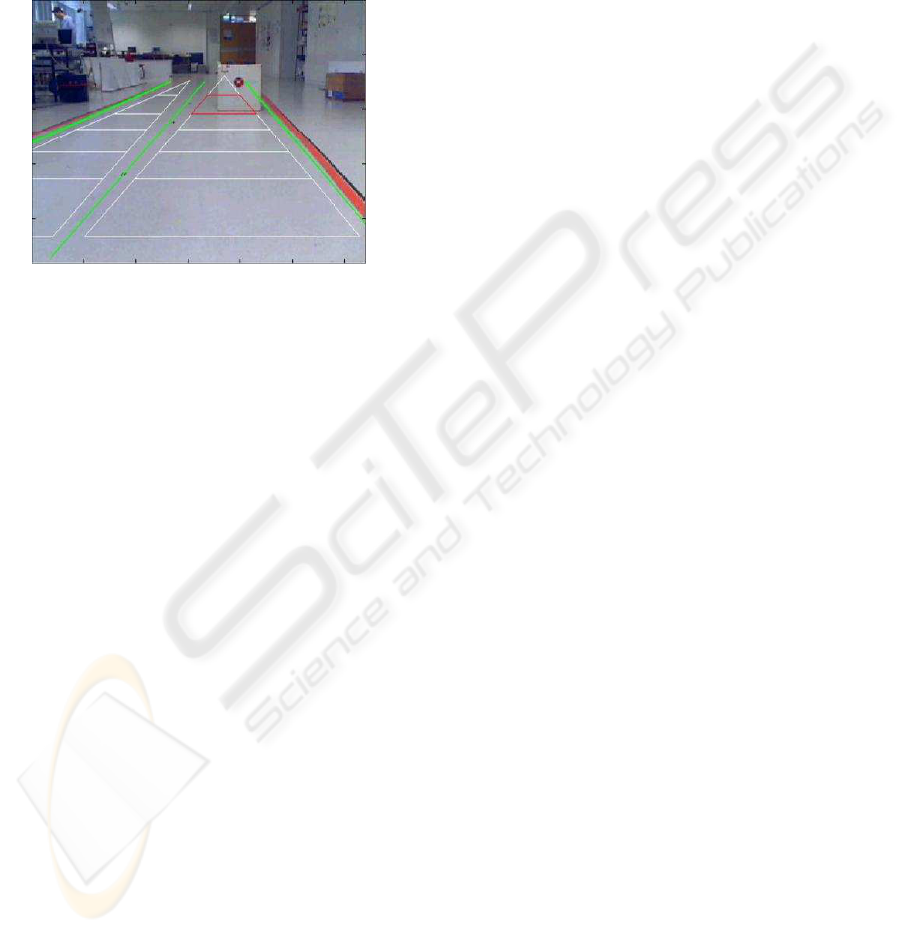
tected side lines. Figure 5 shows the detection of the
lines in the laboratory environment using the above
procedure
Figure 5: Detection of the road limiting lines.
Vehicles lying ahead in the road are detected
through edge detection during the above line search-
ing procedure. The underlying assumption is that any
vehicle has significant edges in an image.
The road ahead the vehicle is divided in a fixed
number of zones. In the image plane these correspond
to the trapezoidal zones, shown in Figure 5, defined
after the road boundary lines and two horizontal lines
at a predefined distance from the robot. A vehicle
is detected in one of the zones when the mean value
of the edges and the percentage of the points inside
the zone that represent edges lie above a predefined
threshold. This value represents a confidence level
that the imaging system detected a vehicle in one of
the zones.
The two values, mean value and percentage value,
represent a simple measure of the intensity and size of
the obstacle edges. These are important to distinguish
between false obstacles in an image. For instance,
arrows painted on the road and the shadow of a bridge,
commonly found in highways, could be detected as an
obstacle or vehicle when doing the image processing.
However, these objects are on the road surface while
a vehicle has a volume. Therefore, an object is only
considered as a vehicle if it is detected in a group of
consecutive zones.
The robot’s lateral position and orientation is de-
termined from the position and slope of the road lines
in the image.
2.3 Fusing Sonar an Image Data
The occupancy grid defined for the representation of
the data acquired by the camera is also used to rep-
resent the obstacle information extracted from the ul-
trasound sensors data. Obstacles lying over a region
of the occupancy grid contribute to the voting of the
cells therein.
Both the camera and ultrasound sensors systems
have associated confidence levels. For the camera
this value is equal to the vehicle detection confidence
level. The sonar confidence level depends on the time
coherence of the detection, meaning that it rises when
a sonar detects a vehicle in the same zone in consec-
utive iterations. The most voted zones in the left and
right lanes are considered as the ones where a vehicle
is detected.
There are areas around the robot which are not
visible by the camera, but need to be monitored be-
fore or during some of the robot trajectories. For in-
stance, consider the beginning of an overtaking ma-
neuver, when a vehicle is detected in the right lane.
The robot can only begin this movement if another
vehicle is not travelling along its left side. Verifying
this situation is done using the information on the po-
sition of the side lines that bound the road and sonar
measurements. If any sonar measurement is smaller
than the distance to the side line the system considers
that a vehicle is moving on the left lane. This method
is also used to check the position of a vehicle that is
being overtaken, enabling to determine when the re-
turn maneuver can be initiated.
3 BEHAVIORS
Safe navigation in a highway consists in the sequen-
tial activation of a sequence of different behaviors,
each controlling the vehicle in the situations arising
in highway driving. These behaviors are such that the
system mimics those of a human driver in similar con-
ditions.
Under reasonably fair conditions, the decisions
taken by a human driver are clearly identified and can
be modeled using a finite state machine. The events
triggering the transition between states are defined af-
ter the data perceived by the sensors. Figure 6 shows
the main components of the decision mechanism used
in this work (note the small number of states). Each
state corresponds to a primitive behavior that can be
commonly identified in human drivers.
Each of these behaviors indicates the desired lane
of navigation. The first behavior, labeled Normal, is
associated with the motion in the right lane, when the
LOW COST SENSING FOR AUTONOMOUS CAR DRIVING IN HIGHWAYS
373
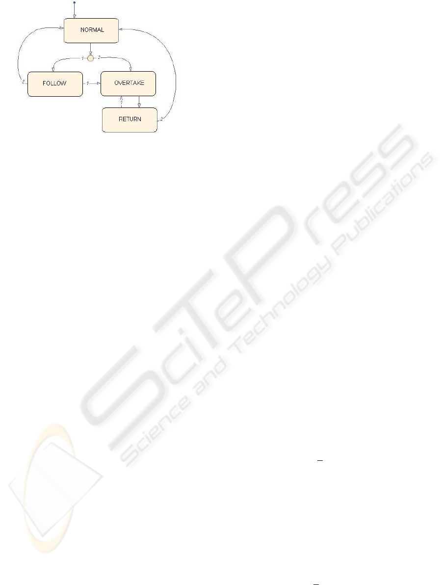
Figure 6: Finite automaton.
road is free. When a vehicle is moving in the right
lane at a smaller speed than the HANS vehicle, the
robot changes to one of two behaviors depending on
the presence of another vehicle in the left lane. If the
lane is clear, the behavior labeled Overtake is trig-
gered and the robot initiates the overtaking maneu-
ver. Otherwise the behavior labeled Follow is trig-
gered and the robot reduces its speed to avoid a col-
lision and follows behind him. The behavior labeled
Return is associated with the return maneuver to the
right lane that concludes the overtaking and is pre-
ceded by checking that the right lane is clear. The last
behaviour, labeled Emergency, not shown in Figure 6,
is activated when an emergency or unexpected situa-
tion is detected and implies an emergency stop, as this
is a safety critical system.
4 ACTUATION
The actuation block receives position references from
the currently active behavior. Assuming safe driving
conditions, the trajectories commonly performed by
vehicles moving in highways are fairly simple.
The control law considered computes the angle
of the steering wheels from a lateral position error
(the horizontal axis in the image plane), (Hong et al.,
2001; Tsugawa, 1999; Coulaud et al., 2006). The ra-
tional under the choice of such a control law is that
for overtaking, and under safe driving conditions, a
human driver sets only a horizontal position reference
while smoothly accelerates its vehicle aiming at gen-
erating a soft trajectory which allows him to change
lane without colliding with the other car. This behav-
ior leads the vehicle to the overtaking lane while in-
creasing the linear velocity relative to the vehicle be-
ing overtaken such that, after a certain time, results
in the overtaking maneuver completed. The refer-
ence for the HANS vehicle is thus a point lying a d
look-ahead-distance, in one of the road lanes. Hard
changes in direction caused by changes in the desired
lane are further reduced through the use of a pre-filter
that smooths the variations of the reference signal.
The control law is then,
ϕ = −Atan
−1
(Ke), (1)
where ϕ is the angle of the directional wheels mea-
sured in the vehicle reference frame e is the lateral
position error, A a constant parameter that is used to
tune the maximum amplitude of ϕ, and K is a constant
parameter used to tune the speed by which the control
changes for a given error. Different values for the pa-
rameters K and A yield different driving behaviors. In
a sense these two parameters allow the tuning of the
macro-behavior of the autonomous driving system.
The primary concern when designing such a sys-
tem must be safety, i.e., the system must operate such
that it does not cause any traffic accident. Under
reasonable assumptions (e.g., any vehicle circulating
does not move on purpose such that is causes an acci-
dent), safety amounts to require system stability. The
overall system is in fact a hybrid system, with the ac-
tive behavior representing the discrete part of the hy-
brid state and the position and velocity of the vehicle
the continuous one. From hybrid systems theory it
is well known that continuous stability of individual
states does not imply stability of the whole system,
i.e., it is not enough to ensure that each behavior is
properly designed to have the global system stable.
Lyapunov analysis can be used to demonstrate that
(1) yields a stable system. Given the HANS vehicle
kinematics (the usual reference frame conventions are
adopted here)
˙x = vsin(θ)cos(ϕ) (2)
˙y = vcos(θ)sin(ϕ)
˙
θ =
v
L
sin(ϕ),
where x,y, θ stand for the usual configuration vari-
ables, v is the linear velocity and L the distance
between the vehicle’s rear and front axis, and the
lateral position and orientation errors, respectively,
e = x + d sin(θ), with d the look-ahead distance, and
ε = θ − θ
0
, after some straightforward manipulation
yields
˙e = V sin(θ+ ϕ)
˙
ε =
V
L
sin(ϕ)
(3)
Substituting in the Lyapunov function candidate
V(e,ε) = 1/2
e
2
+ ε
2
yields for
˙
V(e,ε)
ICINCO 2007 - International Conference on Informatics in Control, Automation and Robotics
374
˙
V = e˙e+ ε
˙
ε = evsin(ε+ ϕ) + ε
v
L
sin(ϕ) (4)
Given that V is positive definite and radially un-
bounded, to have the Lyapunov conditions for global
assymptotic stability verified amounts to verify that
˙
V
is negative definite. Table 5 shows the conditions to
be verified for (4) to be negative.
Case
State variables 1st term 2nd term
1 e > 0, ε > 0 ϕ < −ε ϕ < 0
2
e > 0, ε < 0 ϕ < −ε ϕ > 0
3
e ><,ε > 0 ϕ > −ε ϕ < 0
4
e ><,ε < 0 ϕ > −ε ϕ > 0
(5)
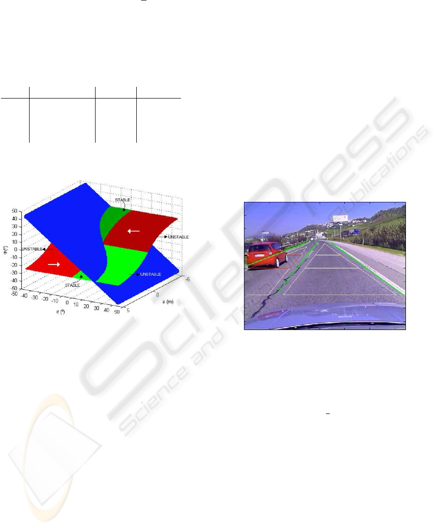
Figure 7 shows the surfaces corresponding to the
third and fourth columns in table 5.
Figure 7: Lyapunov analysis.
Clearly, there are subspaces of the state space for
which the control law (1) does not results in the can-
didate function being a Lyapunov function. However,
the state trajectories when the HANS vehicle lies in
these regions can be easily forced to move towards
the stability regions. For instance, in cases 2 and
3 the vehicle has an orientation no adequate to the
starting/ending of an overtaking maneuver. By sim-
ply controlling the heading of the vehicle before start-
ing/ending the overtaking maneuver, the system state
moves to the subspaces corresponding to situations
1/4, from which (1) yields a stable trajectory.
The analysis above does not demonstrate global
assymptotic stability for the hybrid system that glob-
ally models the HANS system. However, assuming
again reasonable conditions, the results in (Hespanha
and Morse, 1999) can be used to claim that, from
a practical point of view, the system is stable. The
rational behind this claim is that driving in a high-
way does not require frequent switching between be-
haviors, which amounts to say that the dwell time
between discrete state transitions tends to be large
enough to allow each of the behaviors entering in a
stationary phase before the next switching occurs. Us-
ing Figure 7, this means that once the system enters a
stability region it stays there long enough to approach
the equilibrium state (e,ε, ˙e,
˙
ε) = (0,0,0,0). Alter-
natively, global assymptotic stability can be claimed
by using the generalized version of Lyapunov sec-
ond method (see for instance (Smirnov, 2002)) which
only requires that the last behavior triggered in any
sequence of maneuvers is stable.
5 RESULTS
The system was tested in two different conditions.
The imaging module was tested in real conditions,
with the camera mounted in front, behind the car’s
windshield. Figure 8 shows the results.
Figure 8: Testing the imaging module in real conditions.
The testing of the system including the motion be-
haviors was conducted in a laboratory environment
using the ATRV vehicle shown in Figure 2. This
robot was controlled through the kinematics transfor-
mation, u = vcos(ϕ), ω =
v
L
sin(ϕ).
In the first test the robot is moving in the right lane
and, after detecting a car travelling in the same lane
at a lower speed, initiates the overtaking maneuver.
Figure 9 shows the resulting trajectory.
While travelling in the right lane, the Normal be-
havior is active. Once the car in front is detected
the robot switches to the Overtake behavior and initi-
ates the overtaking maneuver moving to the left lane.
Since the velocity of the robot is greater than that of
the car being overtaken, after a while the Perception
block detects that the car is behind the robot and de-
cision system switches to Return. When the centre of
the right lane is reached, the active behavior returns
to Normal completing one cycle of the decision finite
state machine.
LOW COST SENSING FOR AUTONOMOUS CAR DRIVING IN HIGHWAYS
375
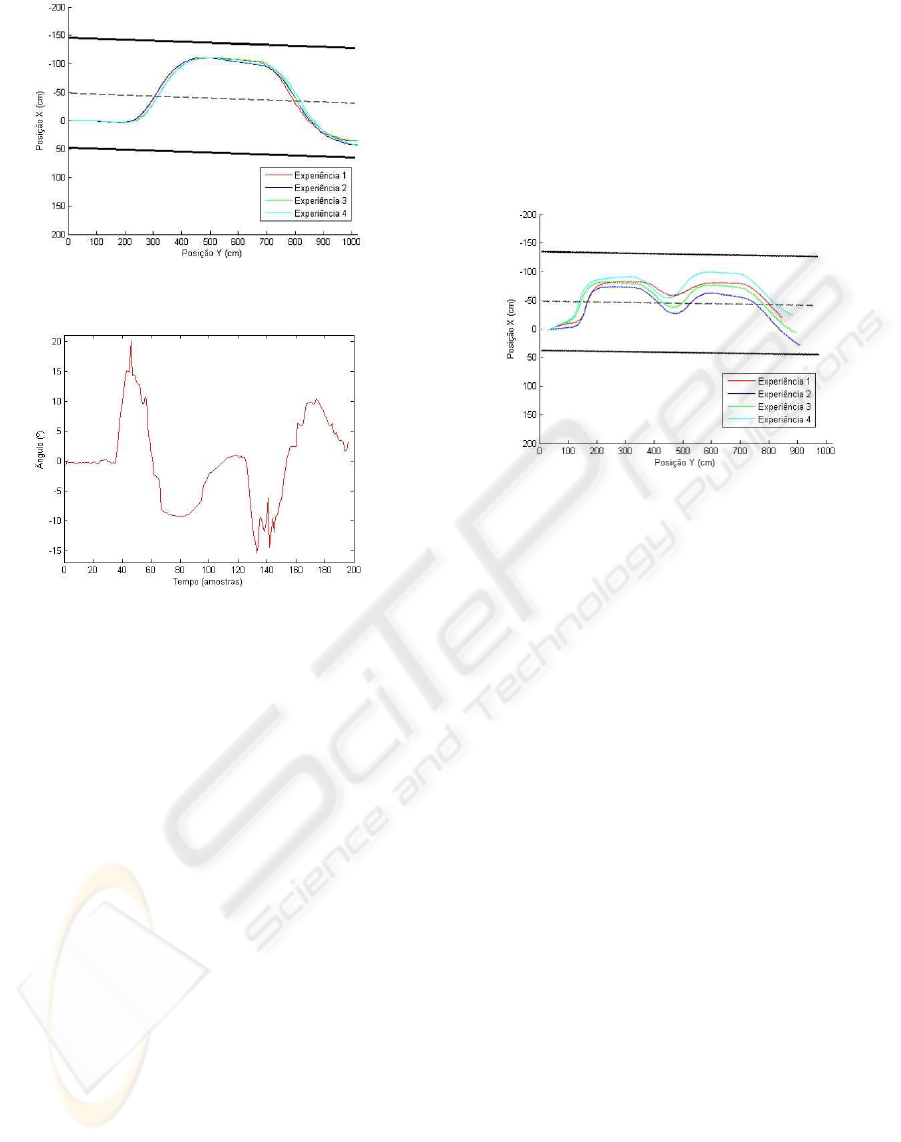
Figure 9: Overtaking a single vehicle.
Figure 10: Steering wheels angle during overtaking.
Figure 10 shows the angle of the steering wheels.
It reaches a maximum around 20
◦
slightly after
switching to Overtake (t = 40), making the robot turn-
ing left, towards the left lane. After reaching the max-
imum direction angle, the lateral error and directional
angle starts decreasing.
Approximately at t = 60 the steering wheels an-
gle is null, meaning that the position of the lookahead
point is at center of the left lane, i.e., the robot is
aligned with the axis of left lane. When ϕ drops to
negative values the robot turns right aiming at reduc-
ing the orientation error and keeping the alignment
with the axis of the left lane. The lane change is com-
pleted at approximately t = 120, when the steering
angle stabilizes at 0, meaning the robot is moving in
the centre of the left lane.
At t = 125 the system switches to the Return be-
havior. The trajectory towards the right lane is similar
(tough inverse) to the one carried out previously from
the right to left lane.
In both lane changes the steering wheel angle is
noisier in the zones where the maximum values are
reached (t = 40 and t = 130). At these moments the
orientation of the robot is high and therefore one of
the road lines (the one farther to the robot) has to be
extrapolated because it is not visible in the camera im-
age. This results in some oscillation in the line’s po-
sition resulting in a noisier position error and steering
wheel angle.
The second experiment aims at verifying the sys-
tem’s response when it is necessary to interrupt an on-
going maneuver to overtake a second vehicle. Figure
11 shows the resulting trajectory.
Figure 11: Double overtaking.
While circulating in the right lane, the robot de-
tects a car in front and initiates the overtaking ma-
neuver following the routine already described in the
previous experiment. When switching to Return the
robot does not detect a second car which is circulating
ahead in the road, in the right lane, at a lower speed.
This situation occurs if the car is outside the HANS’
detection area but inside the area it needs to complete
the return maneuver. If the car was inside the detec-
tion area, HANS would continue along the left lane
until passing by the second car and then return to the
right lane. In this situation, however, the car is only
detected when the robot is approximately in the mid-
dle of the return phase (and of the road). Immediately,
the decision system changes the behavior to Overtake,
the robot initiates a new overtaking maneuver. After
passing by the car, the robot returns to the right lane
to conclude the double overtaking maneuver.
Figure 12 shows the evolution of the steering
wheels angle. The switching from Return to Over-
take) is visible around instant 125 through the drastic
change in the control signal from -18 to 15 degrees.
Still, the system performs a smooth trajectory.
6 CONCLUSION
Despite the low resolution of the chosen sensors, the
perception block was able to generate a representation
of the surrounding environment with which decisions
could be made towards a safe autonomous navigation.
ICINCO 2007 - International Conference on Informatics in Control, Automation and Robotics
376

Figure 12: Steering wheels angle during the double over-
taking.
Obviously, the use of additional sensors, such as more
cameras and laser range finders, would give the sys-
tem enhanced capabilities. Still, the experiments pre-
sented clearly demonstrate the viability of using low
cost sensors for autonomous highway driving of auto-
mobile vehicles.
The sonar data processing uses crude filtering
techniques, namely the occupancy grid and the vot-
ing system, to filter out data outliers such as those
arising due to reflection of sonar beams. Similarly
with image processing, supported in basic techniques
that nonetheless where shown effective, with the line
search based on the edge detection showing robust-
ness to lighting variations.
The small number of behaviours considered was
shown enough for the most common highway driv-
ing situations and exhibit a performance that seems to
be comparable to human. Nevertheless, the decision
system can cope easily with additional behaviors that
might be found necessary in future developments. For
instance, different sets of A,K parameters in (1) yield
different behaviors for the system.
Future work includes the use of additional low
cost cameras and the testing of alternative control
laws, for instance including information on the veloc-
ity of the vehicles driving ahead.
ACKNOWLEDGEMENTS
This work was supported by Fundac¸
˜
ao para a
Ci
ˆ
encia e a Tecnologia (ISR/IST plurianual fund-
ing) through the POS
Conhecimento Program that in-
cludes FEDER funds.
REFERENCES
Broggi, A., Bertozzi, A. Fascioli, A., and Guarino, C.
(1999). The Argo autonomous vehicles vision and
control systems. Int. Journal on Intelligent Control
Systems (IJICS), 3(4).
Canny, J. (1986). A computational approach to edge de-
tection. IEEE Trans. Pattern Analysis and Machine
Intelligence, 8(6):679–698.
Coulaud, J., Campion, G., Bastin, G., and De Wan, M.
(2006). Stability analysis of a vision-based control
design for an autonomous mobile robot. IEEE Trans.
on Robotics and Automation, 22(5):1062–1069. Uni-
versit Catholique de Louvain, Louvain.
Dickmanns, E. (1999). Computer vision and highway au-
tomation. Journal of Vehicle System Dynamics, 31(5-
6):325–343.
Elfes, A. (1989). Using occupancy grids for mobile robot
perception and navigation. Computer, 22(6):46–57.
EUROSTAT (Accessed 2006).
http://epp.eurostat.ec.europa.eu.
Graham, R. (1972). An efficient algorithm for determin-
ing the convex hull of a finite planar set. Information
Processing Letters, 1:132–133.
Hespanha, J. and Morse, A. (1999). Stability of switched
systems with average dwell-time. In Procs of 38th
IEEE Conference on Decision and Control, pages
2655–2660.
Hong, S., Choi, J., Jeong, Y., and Jeong, K. (2001). Lateral
control of autonomous vehicle by yaw rate feedback.
In Procs. of the ISIE 2001, IEEE Int. Symp. on Indus-
trial Electronics, volume 3, pages 1472–1476. Pusan,
South Korea, June 12-16.
Jochen, T., Pomerleau, D., B., K., and J., A. (1995). PANS -
a portable navigation platform. In Procs. of the IEEE
Symposium on Intelligent Vehicles. Detroit, Michigan,
USA, September 25-26.
Smirnov, G. (2002). Introduction to the Theory of Differ-
ential Inclusions, volume 41 of Graduate Studies in
Mathematics. American Mathematical Society.
Thrun, S., Montemerlo, M., Dahlkamp, H., Stavens, D.,
Aron, A., Diebel, J., Fong, P., Gale, J., Halpenny,
M., Hoffmann, G., Lau, K., Oakley, C., Palatucci, M.,
Pratt, V., Stang, P., Strohband, S., Dupont, C., Jen-
drossek, L., Koelen, C., Markey, C., Rummel, C., van
Niekerk, J., Jensen, E., Alessandrini, P., Bradski, G.,
Davies, B., Ettinger, S., Kaehler, A., Nefian, A., and
Mahoney, P. (2006). Stanley: The robot that won the
DARPA Grand Challenge. Journal of Field Robotics,
23(9):661–692.
Tsugawa, S. (1999). An overview on control algorithms for
automated highway systems. In Procs. of the 1999
IEEE/IEEJ/JSAI Int. Conf. on Intelligent Transporta-
tion Systems, pages 234–239. Tokyo, Japan, October
5-8.
Whittaker, W. (2005). Red Team DARPA Grand Challenge
2005 technical paper.
LOW COST SENSING FOR AUTONOMOUS CAR DRIVING IN HIGHWAYS
377
