
Direct and Indirect Classification of High-Frequency
LNA Performance using Machine Learning Techniques
Peter C. Hung, Seán F. McLoone, Magdalena Sánchez
Ronan Farrell and Guoyan Zhang
Institute of Microelectronics and Wireless Systems, Department of Electronic Engineering
National University of Ireland Maynooth, Maynooth, Co. Kildare, Ireland
Abstract. The task of determining low noise amplifier (LNA) high-frequency
performance in functional testing is as challenging as designing the circuit itself
due to the difficulties associated with bringing high frequency signals off-chip.
One possible strategy for circumventing these difficulties is to attempt to pre-
dict the high frequency performance measures using measurements taken at
lower, more accessible, frequencies. This paper investigates the effectiveness of
machine learning based classification techniques at predicting the gain of the
amplifier, a key performance parameter, using such an approach. An indirect
artificial neural network (ANN) and direct support vector machine (SVM) clas-
sification strategy are considered. Simulations show promising results with both
methods, with SVMs outperforming ANNs for the more demanding classifica-
tion scenarios.
1 Introduction
In recent years, functional testing of radio frequency integrated circuits (RFIC) has
faced great challenges, especially for multi-gigahertz RF components. Two main
problems exist: relaying the multi-gigahertz RF signal to the external tester without
affecting the performance of tested RF circuits; building RF production testers operat-
ing in the gigahertz range that are not prohibitively expensive. While advances in
technology and market requirements have seen rapid growth in high-frequency and
high integration RFIC designs, testing practice has not followed suit. Indeed, reliable
high-frequency testing has become the dominant factor in the cost and time-to-market
of novel wireless products [1]. Consequently, developing cost-efficient testing solu-
tions is becoming an increasing important research topic [2-4]. Some of the proposed
schemes for RFIC testing are based on an end-to-end strategy in which the output of
the transmitter and the input of the receiver are linked through a loop-back connec-
tion. In this configuration, the testing of the complete system is carried out without
any external stimulus by employing the on-chip digital hardware available. Unfortu-
nately, this solution is not always applicable to all kinds of RF components. Other
recent proposals for RF system testing have focused on the development of method-
ologies and algorithms for automated test, and Design for Testability (DfT). In Built-
C. Hung P., F. McLoone S., Sánchez M., Farrell R. and Zhang G. (2007).
Direct and Indirect Classification of High-Frequency LNA Performance using Machine Learning Techniques.
In Proceedings of the 3rd International Workshop on Artificial Neural Networks and Intelligent Information Processing, pages 66-75
DOI: 10.5220/0001634500660075
Copyright
c
SciTePress
In-Test (BIT), for example, additional circuitry is included that allows high frequency
tests to be performed on-chip and then evaluated using lower frequency or DC exter-
nal testers [3-5]. However, when considering BIT testing, issues such as area over-
head for embedding and BIT power consumption can add significantly to the cost of
design.
In this paper a different approach is considered. Since many RFICs show strong
correlation between their responses to circuit parameter variation at different frequen-
cies, it is hypothesised that knowledge of responses at lower frequencies may provide
sufficient information to allow classification of responses at higher frequencies.
To investigate this hypothesis, testing of a low noise amplifier (LNA), a key com-
ponent in modern telecommunication systems, is used as a case study. A standard 2.4
GHz design, simulated in ADS® using UMC’s 0.18 μm silicon process technology,
provided the data for our experiments [6]. The LNA circuit consisted of 2 bias tran-
sistors (0.18 μm channel length), 4 RF transistors (0.5 μm channel width), 4 resistors,
3 capacitors and 4 inductors and was deemed to be functioning correctly if the value
of S
21
@ 2.4 GHz was in the range 14.7 dB to 17.2 dB and faulty otherwise. S
21
, a
critical RF circuit performance measure, is essentially the gain of the amplifier.
Random circuit parameter perturbations representative of typical manufacturing
process variations were generated and the value of S
21
recorded at different frequen-
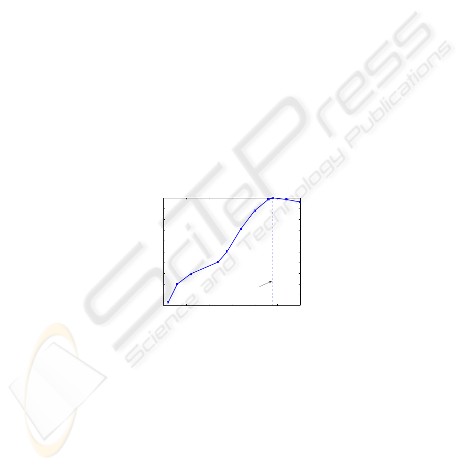
cies. Fig. 1 shows a plot of the correlation that exists between variations in gain (S
21
@ 2.4 GHz) and variations in the same parameter computed at other frequencies.
There is a strong, but decreasing, correlation evident as the circuit excitation fre-
quency moves away from the operating frequency.
Fig. 1. Correlation coefficients between S
21
value computed at different frequencies to the
value computed at the target frequency (2.4 GHz).
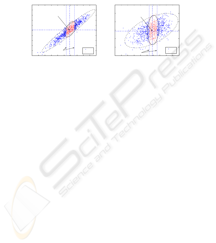
Even when the correlation is high, circuit performance classification on the basis
of these lower frequencies is not straightforward, as demonstrated in Fig. 2. This
shows the relationship between S
21
@ 2.4 GHz and the values computed at: (a) 2.0
GHz and (b) 0.1 GHz, respectively, and highlights the fact that even when the corre-
lation is greater than 90% it is not possible to discriminate between the ‘good’ and
‘bad’ circuits effectively. In fact, simple thresholding on the basis of S
21
@ 2.0 GHz
leads to a misclassification rate of greater than 20%. The misclassification rate in-
creases rapidly as the frequency is reduced and reaches 43.6% for S
21
@ 0.1 GHz.
0 0.5 1 1.5 2 2.5 3
0.5
0.55
0.6
0.65
0.7
0.75
0.8
0.85
0.9
0.95
1
Frequency (GHz)
Correlation Coefficient
2.4 GHz
67
The rapid deterioration in performance is a result of the localised influence of some
parameter variations and the complex nonlinear interaction between circuit compo-
nents.
4 6 8 10 12 14 16 18 20 22 24
4
6
8
10
12
14
16
18
20
22
24
S21@2.4 GHz (dB)
S21@2.0 GHz (dB)
samples of bad/good distribution (data corr. coef. = 0.94052)
bad
good
Nomimal
value
Limits of ’good’
samples
4 6 8 10 12 14 16 18 20 22 24
−70
−65
−60
−55
−50
−45
−40
S21@2.4 GHz (dB)
S21@0.1 GHz (dB)
samples of bad/good distribution (data corr. coef. = 0.5136)
bad
good
Limits of ’good’
samples
Nomimal
value
(a) 2.0 GHz (b) 0.1 GHz
Fig. 2. S
21
parameter relationships for the 2.4 GHz LNA model used in circuit simulations: (a)
S
21
@ 2.0 GHz and (b) S
21
@ 0.1 GHz plotted against S
21
at the operating frequency.
Since the shape of the frequency response of an LNA is a deterministic nonlinear
function of its component parameters, better classification performance can be ex-
pected if the information from several low frequency measurements can be combined.
To that end, this paper considers the possibility of classifying circuit performance
using machine learning techniques. Two strategies are investigated. In the first, an
Artificial Neural Network (ANN) is trained to predict the value of S
21
@ 2.4 GHz
from the values measured at other frequencies and then a thresholding rule is applied
to this prediction to perform the circuit classification, while in the second, a Support
Vector Machine (SVM) is trained to directly classify circuit performance on the basis
of the low frequency S
21
measurements. These two machine learning techniques and
the LNA classification methodology are introduced in Section 2. The simulation
study is then described in Section 3 followed by the results in Section 4. Finally, the
conclusions of the study are presented in Section 5.
2 Machine Learning LNA Performance Classification
Defining the set of N low-frequency S
21
measurements of the i
th
LNA circuit as the
feature vector
i
x (row vector) and the corresponding class label
i
y , with 1+=
i
y
indicating ‘good’ and
1−=
i
y indicating ‘bad’, we can generate a set of L training
data examples,
N
LLii
yyy ℜ∈= ),(),,(),,(),(
11
xxxyX …… ,
(1)
with which to train a classifier to estimate a decision function
68

}1{:)( ±→ℜ
N
f x
(2)
that can then be used to classify new LNA circuits. Here, ‘good’ and ‘bad’ are deter-
mined by a threshold function, z
th
applied to S
21
@ 2.4 GHz, that is
⎩
⎨
⎧
−
<<+
=
otherwise1
17.2 14.7 if1
)(
th
x
xz
(3)
The decision function in (2) can be estimated directly from the training data by using,
for example, a SVM classifier. Alternatively it can be estimated indirectly by first
predicting the value of S
21
@ 2.4 GHz from the feature vector,
GHz4.2@)(
21
Sg →x ,
(4)
and then using a threshold function to perform the classification, that is
}1{))(( :)(
th
±
→xx gzf .
(5)
An ANN such as a Multilayer Perceptron can be used to learn the nonlinear mapping
represented by (4).
2.1 Support Vector Machines (SVM)
SVMs, first proposed by Vladimir Vapnik in 1963 [7], are a supervised linear learn-
ing technique widely used for classification problems. They are known to perform
binary classification well in many practical applications. Consider a separating hyper-
plane that divides two classes of data:
ℜ∈ℜ∈=−⋅ bb
N
,,0 wxw ,
(6)
where w and
b are unknown coefficients, and two additional hyperplanes that are
parallel to the separating hyperplane:
1
1
−=−⋅
=
−
⋅
b
b
xw
xw
(7)
Defining the margin as the perpendicular distance between the parallel hyperplanes,
the optimal hyperplane is the one which results in the maximum margin of separation
between the two classes. Mathematically the problem can be expressed as
Liby
ii
,,2,1,1)(tosubject),(min
2
max …=≥−⋅⋅≡ xwww
w
w
w
.
(8)
This is a constrained quadratic optimisation problem whose solution
w
has an ex-
pansion [8]
∑
=
i
ii
v xw ,
(9)
69

where
i
x are the subset of the training data, referred to as support vectors, located on
the parallel hyperplanes, and
i
v are the corresponding weighting factors. The linear
SVM (LSVM) decision function is then given by
)()(
SVMLSVM
bzf
−
⋅
=
xwx
(10)
where
SVM
z is defined as
⎩
⎨
⎧
<−
≥+
=
0if1
0if1
)(
SVM
φ
φ
φ
z
(11)
The decision function in Eq. (10) can be rewritten as
⎟
⎟
⎠
⎞
⎜
⎜
⎝
⎛
−⋅=
∑
bvzf
i
ii
)()(
SVMLSVM
xxx
(12)
with the result that it is only dependent on dot products between the test data vector,
x, and the support vectors. This important property allows SVMs to be extended to
problems where nonlinear partitions of data sets are required. This is achieved by
replacing the dot products by a kernel function
(.)k which meets the Mercer’s condi-
tion [9]:
)()(),(
jiji
k xxxx Φ⋅Φ=
,
(13)
thereby mapping the data into a higher dimension feature space where linear SVM
classification can be performed. Note the resulting decision function, in the original
data space, will be nonlinear and takes the form
(
)
rzf
SVMSVM
)( =x
, where
∑
−=
L
i
ii
bkvr ),(. xx
(14)
In non-separable problems where different classes of data overlap, slack variables
can be introduced so that a certain amount of training error or data residing within the
margin is permitted. This gives rise to a ‘soft margin’ optimisation function [9, 10].
To give users the ability to adjust the amount of training error allowed in the optimi-
sation, a smoothing parameter
C
is incorporated into the soft margin function, with a
larger
C
corresponding to assigning a larger penalty to errors.
The Gaussian radial basis function (RBF) defined as
⎟
⎟
⎟
⎠
⎞
⎜
⎜
⎜
⎝
⎛
−
−=
2
2
RBF
2
exp),(
σ
ji
ji
k
xx
xx
(15)
is a popular choice of SVM kernel and the one selected for this application. The pa-
rameter,
σ
, controls the width of the kernel and is determined as part of the classifier
training process.
70

2.2 Artificial Neural Networks
Neural networks [11] are one of the best known and most commonly-used machine
learning techniques. There are various configurations and structures of NNs, but all
contain an array of neurons that are linked together, usually in multiple layers. In this
application a single hidden layer Multilayer Perceptron (MLP) topology is chosen
because of its universal function approximation capabilities, good generalisation
properties and the availability of robust efficient training algorithms [12].
The output of a single hidden layer MLP can be written as a linear combination of
sigmoid functions (i.e. neurons),
(
)
∑
+=
i
i
h
i
h
sigwbg xwx ),(
NN
,
(16)
where
)exp(1
1
)(
u
i
u
i
i
b
sig
+⋅+
=
xw
x
.
(17)
Here,
h
i
w
,
u
i
w
,
u
i
b
,( Mi ,,2,1 = ) and
h
b are weights and biases which collectively
form the network weights vector,
NN
w . Defining a Mean Squared Error (MSE) cost
function over the training data
2
1
NNNN
)),((
1
)(
p
L
p
p
dg
L
E −=
∑
=
wxw ,
(18)
with
p
d
corresponding to the desired network output for the p
th
training pattern (i.e.
S
21
@ 2.4 GHz), the optimum weights can be determined using gradient based opti-
misation techniques.
3 Simulation Study
To evaluate the potential for employing multiple low frequency S
21
measurements to
classify LNA S
21
performance at 2.4 GHz and to compare the performance of the
proposed machine learning classifiers, a Monte Carlo simulation study was under-
taken using a 2.4 GHz LNA model implemented in ADS®. Uniform random varia-
tions were introduced into 38 of the model parameters to represent typical LNA
manufacturing process variations and 10,000 circuit simulations performed. While in
practice circuit parameters might be expected to vary normally around their nominal
values, uniform distributions were chosen to give an even coverage of the LNA pa-
rameter space. Catastrophic failures, such as short-circuits, were not considered as
these can be identified relatively easily using existing IC testing techniques.
For each circuit the S
21
performance parameter was recorded at 0.1, 0.3, 0.6, 1.2,
1.4, 1.7 and 2.0 GHz and also at the operating frequency (2.4 GHz). This data was
71

then normalised to have zero mean and unit variance and divided into training and
test data sets, each containing 5,000 samples.
Two different feature vectors were considered in the study, containing S
21
meas-
urements up to 1.4 GHz and 2.0 GHz, respectively, that is:
]S,S,S,S,S[
4.1
21
2.1
21
6.0
21
3.0
21
1.0
214.1
=x
(19)
and
]S,S,S,S,S,S,S[
0.2
21
7.1
21
4.1
21
2.1
21
6.0
21
3.0
21
1.0
210.2
=x .
(20)
Here,
f
21
S denotes the value of S
21
at f GHz. In each case the target MLP model out-
put is
4.2
21
S
while the target labels for the SVM classifier are given by
)S(
4.2
21th
z
.
3.1 MLP Training
MLP training was performed using the hybrid BFGS training algorithm [12] with
stopped minimisation used to prevent over-fitting [13]. The optimum number of neu-
rons (M ) was determined for each model by systematically evaluating different net-
work sizes and selecting the network with the minimum MSE on the test data set.
Training was repeated ten times for each network size to allow for random weight
initialisations and the best set of weights recorded in each case.
The optimum network sizes and resulting model fit, measured in terms of the cor-
relation with the true value of
4.2
21
S , are summarised in Table 1. For comparison pur-
poses, the correlation between
4.2
21
S and the measurements at 1.4 and 2.0 GHz are also
given.
Table 1. Optimum MLP classifier model dimensions and resulting model fit.
Feature vector Network dimensions Model fit
4.1
x
MLP(5,12,1) 0.9364
0.2
x
MLP(7,15,1) 0.9979
4.1
21
S
- 0.7537
0.2
21
S
- 0.9408
As expected, the exploitation of multiple frequencies results in much better pre-
dictability of
4.2
21
S than using the measurement at a single frequency. Notably, the
information provided by
0.2
21
S is still marginally greater than the combined information
provided by all measurements up to 1.4 GHz. The classification performance of these
networks, when employed in the indirect LNA classifier scheme, will be reported in
Section 4.
72
3.2 SVM Training
SVM training was performed using the Matlab® package simpleSVM [14]. The ker-
nel width parameter
σ
and smoothing parameter C were fine tuned manually and
optimised on the basis of classification performance on the test data set. The final
values selected were
9.0=
σ
and 000,100
=
C .
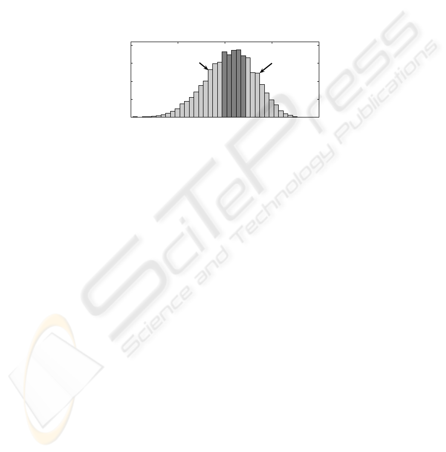
Initial SVM results were quite poor despite expectations of superior performance
to indirect classification using MLPs (results presented in Section 4). It was deter-
mined that this was due to the bimodal distribution of the out-of-specification circuits
forming the ‘bad’ class, i.e. it consists of two segments separated by the ‘good’ class,
as shown in Fig. 3.
5 10 15 20 25
0
200
400
600
800
S
21
@ 2.4 GHz (dB)
Historgram Frequency
Good
Bad lower
Bad upper
Fig. 3. Histogram of ‘good’ and ‘bad’ circuits as defined by the S
21
performance criteria.
The a priori knowledge of the distribution of the ‘bad’ circuits can be taken into
account by splitting the ‘bad’ samples into ‘bad lower’ and ‘bad upper’ samples,
thereby introducing 3 classes – ‘bad lower’, ‘good’ and ‘bad upper’. SVM classifica-
tion is then performed in two-stages. Firstly, two binary SVMs are trained, one to
classify LNAs as either ‘bad lower’ or ‘not bad lower’, and one to classify LNAs as
either ‘bad upper’ or ‘not bad upper’. Then the overall classification is obtained from
a weighted linear combination of the individual decision functions, that is:
)(
BUBLSVMSVM3
rKrzf
+
=
.
(21)
Here,
r
is as defined in Eq. (14), subscripts BL and BU represent the ‘bad lower’ and
‘bad upper’ classifiers and the constant
K
is a scalar which is chosen to maximise
the correlation between
SVM3
f and the true class labels over the training data.
This 3-class SVM approach is denoted SVM3 while the original two class SVM
classifier will be referred to as SVM2.
4 Results
The performance of the MLP, SVM2 and SVM3 LNA classifiers was measured in
terms of the following metrics computed on the test data set:
GPR: good pass rate - Percentage of good LNAs passed;
BFR: bad fail rate - Percentage of bad LNAs failed;
FR: failure rate - Percentage of passed LNAs incorrectly classified as ‘good’;
73

MCR: misclassification rate - Percentage of LNAs incorrectly classified.
Since the good pass rate (GPR) and bad fail rate (BFR) of a classifier vary as a func-
tion the classification threshold, with one increasing as the other deceases, the thresh-
old can be adjusted to control one or other of these metrics. Here, the threshold of
each classifier was adjusted to give a fixed BFR, reflecting the importance in the
electronics industry of controlling the number of faulty components released to the
market.
Table 2 shows the mean performance of each classifier when their thresholds were
selected to give a BFR of 90% and 75%, respectively. The result for classification on
the basis of single frequency measurements at 1.4 and 2.0 GHz are also included for
comparison. To provide robust estimates, the metrics were computed by averaging
over 100 batches of LNAs generated from the test data set using sampling with re-
placement. Each batch consisted of 500 ‘good’ and 500 ‘bad’ circuits randomly se-
lected (with replacement) from a total of 1,795 ‘good’ and 3,205 ‘bad’ examples in
the data set.
Table 2. Mean performance of the MLP, SVM2 and SVM3 LNA classifiers.
BFR (%)
90 75
Inputs
Method
GPR
(%)
FR
(%)
MCR
(%)
GPR
(%)
FR
(%)
MCR
(%)
MLP 57.11 14.88 26.45 81.03 23.55 21.99
x
1.4
SVM2 44.18 18.43 27.96 77.32 24.41 11.39
SVM3
82.30
10.82 13.85
90.85
21.56 17.08
MLP
99.70
9.09 5.15
100.00
19.97 12.50
x
2.0
SVM2 84.40 10.57 12.80 97.33 20.41 13.83
SVM3 97.60 9.28 6.20 99.34 20.09 12.83
4.1
21
S
- 19.98 33.29 45.01 47.13 34.63 38.94
0.2
21
S
- 55.48 15.24 27.27 84.65 22.78 20.17
Comparing the different classifiers, it can be seen that SVM3 provides the most
consistent performance. Although the MLP classifier produces the best results when
using frequencies up to 2.0 GHz, SVM3 is only around 2% and 0.7% behind. More
importantly, when LNA classification is performed using S
21
measurements up to 1.4
GHz only, SVM3 outperforms the MLP solution by 25% and 9% respectively. It is
noted that high GPRs are always accompanied by correspondingly low values of FR
and MCR. As expected, the performance of all classifiers deteriorates when only the
lower frequency S
21
measurements (x
1.4
) are considered, though SVM3 and MLP still
outperform the classifications obtained using a single S
21
measurement at 2.0 GHz.
Interestingly, the SVM classifier was only able to outperform the MLP classifier
when the a priori knowledge of the bimodal distribution of the out-of-specification
LNAs was taken into account. In all cases SVM2 is substantially inferior to both the
MLP and SVM3 classifiers. This suggests that while SVMs are the natural setting for
classification they do not always yield the optimum results.
Although this study does not consider catastrophic IC failures, they can be identi-
fied relatively easily using other simple tests such as supply current tests. Overall, the
results successfully demonstrate the usefulness of machine learning techniques for
74

LNA functional testing. For example, it can lower the cost of testing by extending
the frequency range of existing ATE testers by as much as 70%.
5 Conclusions
Functional testing of high-frequency LNAs is becoming a prohibitively expensive
and time-consuming exercise, due to the difficulties with bringing such signals off-
chip. This paper proposes a novel testing strategy in which machine learning classifi-
ers are used to predict high-frequency LNA performance by combining information
from several lower frequency measurements. Promising results are obtained using
both direct SVM and indirect MLP classifiers.
Acknowledgements
The authors gratefully acknowledge the financial support of Enterprise Ireland.
References
1. Ferrario, J., Wolf, R., Ding, H.: Moving from mixed signal to RF test hardware develop-
ment. IEEE Int. Test Conference (2001) 948–956
2. Lau, W. Y.: Measurement challenges for on-wafer RF-SOC test. 27th Annual IEEE/SEMI
Int. Elect. Manufact. Tech. Symp. (2002) 353–359
3. Negreiros, M., Carro, L., Susin, A.: Low cost on-line testing of RF circuits. 10th IEEE Int.
On-Line Testing Symp. (2004) 73–78
4. Doskocil, D. C.: Advanced RF built in test. AUTOTESTCON '92 IEEE Sys. Readiness
Tech. Conf. (1992) 213–217
5. Goff, M. E., Barratt, C. A.: DC to 40 GHz MMIC power sensor. Gallium Arsenide IC
Symp. (1990) 105–108.
6. Allen, P. E., Holberg, D. R.: CMOS analog circuit design. 2nd edn. Oxford University
Press, Oxford (2002)
7. Vapnil V., Lerner A.: Pattern recognition using generalised portrait method. Automation
and Remote Control 24 (1963)
8. Hearst, M.A.: SVMs – a practical consequence of learning theory. IEEE Intelligent Sys.
(1998) 18–21
9. Burges, C. J.: A tutorial on support vector machines for pattern recognition. Data Mining
and Knowledge Discovery 2 (1998) 121–167
10. Cortes C., Vapnik V.: Support vector networks. Machine Learning 20 (1995) 273–297
11. Haykin, S.: Neural Networks: A comprehensive foundation. 2nd edn. Prentice Hall, New
Jersey (1998)
12. McLoone S., Brown M., Irwin G., Lightbody G.: A hybrid linear/nonlinear training algo-
rithm for feedforward neural networks. IEEE Trans. on Neural Networks 9 (1998) 669-684
13. Sjöberg, J., Ljung, L.: Overtraining, regularization, and searching for minimum with appli-
cation to neural networks. Int. J. Control 62 (1995) 1391-1407
14. Vishwanathan S. V. N., Smola A. J., Murty M. N.: SimpleSVM. Proc. 20th Int. Conf.
Machine Learning (2003)
75
