
PROBABILISTIC MAP BUILDING CONSIDERING SENSOR
VISIBILITY
Kazuma Haraguchi, Jun Miura
Department of Computer-Controlled Mechanical Systems, Graduate School of Engineering, Osaka University
2-1 Yamadaoka, Suita, Osaka, Japan
Nobutaka Shimada, Yoshiaki Shirai
Department of Computer Science Faculty of Science Engineering Ritsumeikan University
1-1-1 Nojihigashi, kusatsu, shiga, Japan
Keywords:
Obstacle Map Generation, Bayes Theorem, Occlusion, Spatial Dependency, Visibility.
Abstract:
This paper describes a method of probabilistic obstacle map building based on Bayesian estimation. Most
active or passive obstacle sensors observe only the most frontal objects and any objects behind them are oc-
cluded. Since the observation of distant places includes large depth errors, conventional methods which does
not consider the sensor occlusion often generate erroneous maps. We introduce a probabilistic observation
model which determines the visible objects. We first estimate probabilistic visibility from the current view-
point by a Markov chain model based on the knowledge of the average sizes of obstacles and free areas.
Then the likelihood of the observations based on the probabilistic visibility are estimated and then the poste-
rior probability of each map grid are updated by Bayesian update rule. Experimental results show that more
precise map building can be bult by this method.
1 INTRODUCTION
The well known SLAM(Simultaneous Localization
And Mapping)(Montemerlo and Thrun, 2002; Thrun
et al., 2004; Grisetti et al., 2005) process could be
divided in two parts: position localization using cur-
rent observations and the current map, and the map
update using the estimated position. This paper dis-
cusses the problem of the conventional map update
methods, sensor occlusion, and proposes a novel up-
dating method solving it.
The positions of landmarks and obstacles should
be represented on the map for navigation(Thrun,
2002b). There are two representations available for
them:
1. Feature point on the obstacle
2. Obstacle existence on small map grid.
Former representation requires feature identification
and matching and the feature position is update when
new observation is available(Suppes et al., 2001).
Latter representation identifies the map grid from
which the observation comes. Since laser range sen-
sors, ultrasonic sensors and stereo image sensors can
precisely control the direction of transmitting and re-
ceiving light or sound, the place from which observa-
tion comes is easy to identify. Thus we use the latter
map representation here.
The obstacle sensor output always includes obser-
vation errors. For example flight time measurement
of light or sound have errors caused by wave refrac-
tion, diffraction and multi-path reflection. Stereo im-
age sensor also has correspondence failures of image
features. These errors lead to large errors or ghost
observations. Therefore the map building should be
established in a probabilistic way based on a certain
error distribution model.
Here we use a probabilistic occupancy grid map
for the map representation, which stores the obstacle
existence probability in each map grid. In this repre-
sentation, the obstacle existence probability of each
grid is updated by evaluating the likelihood of ob-
tained observation for the grid and integrate it with its
prior probability in the way of Bayesian estimation.
While a generic solution of this map building for-
mulation is solved by Markov Random Field (MRF)
200
Haraguchi K., Miura J., Shimada N. and Shirai Y. (2007).
PROBABILISTIC MAP BUILDING CONSIDERING SENSOR VISIBILITY.
In Proceedings of the Fourth International Conference on Informatics in Control, Automation and Robotics, pages 200-206
DOI: 10.5220/0001623502000206
Copyright
c
SciTePress
observation
distribution of obstacle
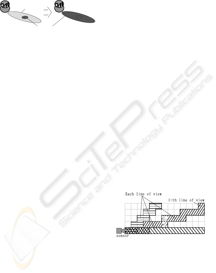
Figure 1: Result of update when the robot gets the observa-
tion of the obstacle of substantial margin of error.
(Rachlin et al., 2005), its computational cost is huge,
especially in case of high grid resolution. Previous
methods (Miura et al., 2002; Thrun, 2002a; Moravec,
1988) use the following assumptions for reduction of
computation:
1. Observation obtained for each map grid is prob-
abilistically independent (it depends on only the
state (obstacle existence) of that grid).
2. Obstacle existence of each map grid is indepen-
dent to each other.
Most obstacle sensors observe the most frontal ob-
jects and any objects behind them are occluded. Since
such sensors having sensor occlusion characteristic
does not satisfy the above assumption 1, the follow-
ing serious problems are caused by forcedly using the
assumption.
As shown in the left side picture of Figure 1, sup-
pose that dark grey ellipsoidal region has higher prob-
ability of obstacle existence than the outside. Then
suppose that the obstacle observation with large error
(ex. distant observation with stereo vision) is obtained
shown as the light grey region in the figure. In that
situation, that observation probably comes from the
most frontal part of the dark grey region. The assump-
tion 1, however, the obstacle existence probability of
each map grid is independently updated by integrat-
ing the observation and it is obviously overestimated.
As a result everywhere distant from the current robot
position tends to be estimated as obstacle in the map.
Therefore the assumption 1 should be rejected.
In addition, the assumption 2 also leads to the
other problems. If the obstacle existence in each map
grid is independent, the probability of that a certain
area is open as free-space is estimated as the product
of the probability of each map grid. This leads to an
obviously irrational result that more precise grid reso-
lution is adopted, abruptly smaller becomes the free-
space probability of the same area (in other words,
the viewing field is more invisible due to occluding
obstacles).
In real scenes, obstacles and free-spaces has a
certain size. This points out the existence of co-
occurrence between the adjacent grids, called spatial
continuity. Since the co-occurrence becomes larger
when the grid resolution is more precise, the free-
space probability can be correctly estimated regard-
less of the grid resolution. Thus the assumption 2 also
should be rejected.
Our map building method correctly considers sen-
sor occlusion and spatial continuity. A certain ob-
stacle is visible if and only if the space between the
sensor and the obstacle is entirely open as free-space.
Therefore we introduce a novel method of estimating
visibility of the obstacle on each map grid by consid-
ering spatial continuity, and updating the obstacle ex-
istence probability with proper consideration of sen-
sor occlusion.
2 MAP BUILDING
CONSIDERING SENSOR
VISIBILITY
2.1 Joint Probability of Adjacent Grids
on Each Viewing Ray
We first divide the map grids into multiple viewing
rays. The sensor observes the existence of obstacle
on each ray. In this paper, we represent the viewing
ray as the 4-connected digital line as shown in Fig-
ure 2. On each ray we consider the probabilistic grid
state (whether obstacle exists on the grid or not) as
a simple Markov chain. Thus each grid state can be
represented as the joint probability of two grid states
adjacent on each ray.
Figure 2: Approximated Lines of view.
We first estimate the joint probability of the jth
and j + 1th grid (the jth grid is nearer to the sensor)
on a viewing ray (see Figure 2). Let e
l
j
=
n
E
l
j
,
¯
E
l
j
o
be
the state of the jth grid on the lth ray (E:occupied by
an obstacle,
¯
E: not occupied), and P(e
l
j
, e
l
j+1
|O) be
the joint probability of the jth and j+ 1th grid under
O, the series of the previous observations. Then the
joint probability after the latest observation o obtained
PROBABILISTIC MAP BUILDING CONSIDERING SENSOR VISIBILITY
201
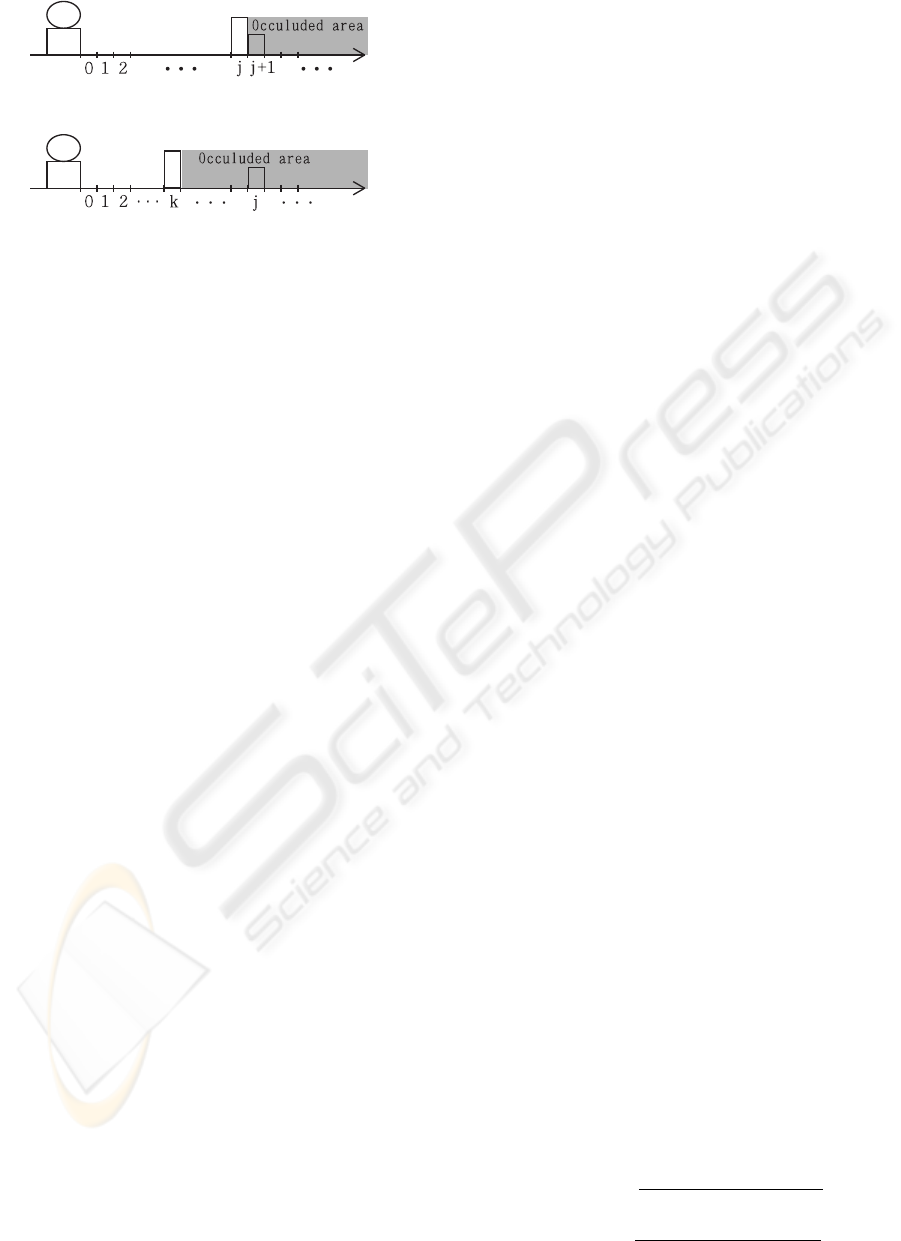
Figure 3: Occluded area behind the j-th grid.
Figure 4: Occluded area behind the k-th grid.
is calculated as :
P(e
l
j
, e
l
j+1
|o, O) = α
l
P(o
l
|e
l
j
, e
l
j+1
, O)P(e
l
j
, e
l
j+1
|O). (1)
o
l
, α
l
, P(e
l
j
, e
l
j+1
|O) and P(o
l
|e
l
j
, e
l
j+1
, O) respectively
denote the observation on the ray l, a normalizing
constant, the prior probability and the likelihood. The
likelihood P(o
l
|e
l
j
, e
l
j+1
, O) should be calculated by
considering the sensor visibility as the following sec-
tion.
2.2 Likelihood Considering Sensor
Visibility
Since an observation on the ray l, o
l
, depends
on grid states just on the the ray, the likelihood
P(o
l
|e
l
j
, e
l
j+1
, O) is calculated as:
P(o
l
|e
l
j
, e
l
j+1
, O) =
∑
m
l
∈Ω
l
P(o
l
|m
l
, e
l
j
, e
l
j+1
, O)P(m
l
|e
l
j
, e
l
j+1
, O)
(2)
where m
l
denotes grid states on the ray l except
e
l
j
,e
l
j+1
. The direct calculation of Eq. 2 requires huge
summation of 2
N
l
order, where N
l
denotes the number
of grids on the ray l.
Actually this calculation is drastically reduced
by considering the sensor visibility. There exist
four cases of the adjacent grid states: (E
j
, E
j+1
),
(E
j
,
¯
E
j+1
), (
¯
E
j
, E
j+1
), (
¯
E
j
,
¯
E
j+1
). In (E
j
, E
j+1
) case
(this means both the grid j and j + 1 are occupied),
since grid j occludes j + 1 as shown in Figure 3, the
likelihood P(o
l
|E
l
j
, E
l
j+1
, O) is no longer dependent
on j+ 1, and then it is represented as
P(o
l
|E
l
j
, E
l
j+1
, O)= P(o
l
|E
l
j
, O). (3)
The above likelihood is acceptable only when grid j is
visible from the sensor, namely whole grids between
the sensor and grid j are empty. If not so, the most
frontal occupied grid k(< j) is observed (see Figure
4). Here, define an stochastic event F
k
as follows:
F
k
=
E
0
(k = 0)
¯
E
0
∩
¯
E
1
∩ ·· · ∩
¯
E
k−1
∩ E
k
(k > 0).
Since F
0
, ··· , F
k
are mutually exclusive events, the
right-hand of Eq.3 is expanded as follows:
P(o
l
|E
l
j
, O)=
j
∑
k=0
P(o
l
|F
l
k
, E
l
j
, O)P(F
l
k
|E
l
j
, O)
=
j
∑
k=0
P(o
l
|F
l
k
)P(F
l
k
|E
l
j
, O) (4)
because o
l
is no longer dependent on any grid behind
grid k nor the previous observations O.
The likelihoods for the rest three cases (E
j
,
¯
E
j+1
),
(
¯
E
j
, E
j+1
), (
¯
E
j
,
¯
E
j+1
), is represented as follows in the
same considerations:
P(o
l
|E
l
j
,
¯
E
l
j+1
, O) =
∑
j
k=0
P(o
l
|F
l
k
)P(F
l
k
|E
l
j
, O) (5)
P(o
l
|
¯
E
l
j
, E
l
j+1
, O) =
∑
j−1
k=0
P(o
l
|F
l
k
)P(F
l
k
|
¯
E
l
j
, O)
+P(o
l
|F
l
j+1
)P(F
l
j+1
|O) (6)
P(o
l
|
¯
E
l
j
,
¯
E
l
j+1
, O) =
∑
j−1
k=0
P(o
l
|F
l
k
)P(F
l
k
|
¯
E
l
j
, O)
+
∑
∞
k= j+1
P(o
l
|F
l
k
)P(F
l
k
|O).(7)
P(o
l
|F
l
k
) in Eqs.(4)-(7) is a sensor kernel model which
defines the measurement error distribution of the sen-
sor observation. This is provided for each kind of sen-
sor. These equations say that the likelihood of grid j
and j+1 is contributed by grid k ahead grid j accord-
ing to P(F
l
k
|E
l
j
, O), P(F
l
k
|
¯
E
l
j
, O), P(F
l
k
|O), which mean
conditional visibilities of grid k.
Since these visibilities are required to be estimated
before the above likelihood calculations, they should
be estimated by calculating the Markov chain because
the actual grid states are not independent due to spa-
tial continuity. The Markov chain is calculated based
on the grid state probabilities (joint probability of e
j
,
and e
j+1
) obtained in the previous time slice:
P(F
l
k
|E
l
j
, O) =P(
¯
E
l
0
|
¯
E
l
1
, O)P(
¯
E
l
1
|
¯
E
l
2
, O)P(
¯
E
l
2
|
¯
E
l
3
, O)
···P(
¯
E
l
k−1
|E
l
k
, O)P(E
l
k
|E
l
j
, O) (8)
P(F
l
k
|
¯
E
l
j
, O) =P(
¯
E
l
0
|
¯
E
l
1
, O)P(
¯
E
l
1
|
¯
E
l
2
, O)P(
¯
E
l
2
|
¯
E
l
3
, O)
···P(
¯
E
l
k−1
|E
l
k
, O)P(E
l
k
|
¯
E
l
j
, O) (9)
P(F
l
k
|O) =P(
¯
E
l
0
|
¯
E
l
1
, O)P(
¯
E
l
1
|
¯
E
l
2
, O)P(
¯
E
l
2
|
¯
E
l
3
, O)
···P(
¯
E
l
k−1
|E
l
k
, O)P(E
l
k
|O) (10)
where P(E
l
k
|O), P(
¯
E
l
k−1
|E
l
k
, O) and P(
¯
E
l
q
|
¯
E
l
q+1
, O)
(0 ≤ q < k − 1) are calculated as follows:
P(E
l
k
|O)= P(E
l
k
, E
l
k+1
|O) +P(E
l
k
,
¯
E
l
k+1
|O)(11)
P(
¯
E
l
k−1
|E
l
k
, O) =
P(
¯
E
l
k−1
,E
l
k
|O)
P(E
l
k−1
,E
l
k
|O)+P(
¯
E
l
k−1
,E
l
k
|O)
(12)
P(
¯
E
l
q
|
¯
E
l
q+1
, O) =
P(
¯
E
l
q
,
¯
E
l
q+1
|O)
P(
¯
E
l
q
,
¯
E
l
q+1
|O)+P(E
l
q
,
¯
E
l
q+1
|O)
. (13)
ICINCO 2007 - International Conference on Informatics in Control, Automation and Robotics
202
i
each neighbor(m-th) cell
Figure 5: Adjacent grids.
P(E
l
k
|E
l
j
, O) and P(E
l
k
|
¯
E
l
j
, O) are also obtained by cal-
culating the Markov chain:
P(E
l
k
, E
l
j
|O)= P(E
l
k
|O)P(E
l
j
|O) + α
k, j
∏
j−1
q=k
c
l
q,q+1
(14)
P(E
l
k
,
¯
E
l
j
|O)= P(E
l
k
|O)P(
¯
E
l
j
|O) − α
k, j
∏
j−1
q=k
c
l
q,q+1
(15)
where
c
l
q,q+1
=
P(E
l
q
,E
l
q+1
|O)−P(E
l
q
|O)P(E
l
q+1
|O)
q
P(E
l
q
|O)P(
¯
E
l
q
|O)P(E
l
q+1
|O)P(
¯
E
l
q+1
|O)
(16)
α
k, j
=
q
P(E
l
k
|O)P(
¯
E
l
k
|O)P(E
l
j
|O)P(
¯
E
l
j
|O).(17)
c
l
q,q+1
means correlation between the adjacent grid
e
l
q
and e
l
q+1
. The grid visibilities are estimated from
Eqs.(8)-(17), then the likelihoods considering sensor
visibility, Eqs.(4)- (7), are calculated. Finally the pos-
teriors, Eq.(1) is updated for each grid.
2.3 Posterior Update Across Viewing
Rays
The grid posteriors for each viewing ray, estimated
in the way of the previous section, conflict with the
posteriors of the adjacent rays, because they actually
have interactions across the rays and the independent
update of each ray is just an approximation. True pos-
teriors should satisfy the following two constraints:
the first one is
∑
e
i
,e
j
∈{E,
¯
E}
P(e
i
, e
j
) ≡ 1 (18)
where grid i and j is adjacent, and the second one is
P(e
i
) ≡ P(e
i
, E
m
) +P(e
i
,
¯
E
m
) (19)
for every grid m adjacent to grid j (see Figure 5).
Therefore we estimate the true posteriors by least
squares method under the constraints Eqs.(18),(19).
The minimised error ∆
2
is written as
∆
2
=
∑
i, j
∑
e
i
,e
j
P
∗
(e
i
, e
j
) −P(e
i
, e
j
)
2
(20)
where P
∗
(e
i
, e
j
) is the conflicting posteriors, P(e
i
, e
j
)
is the estimated posteriors satisfying the constraints.
This minimization is easily solved by Lagrange’s
method in low cost.
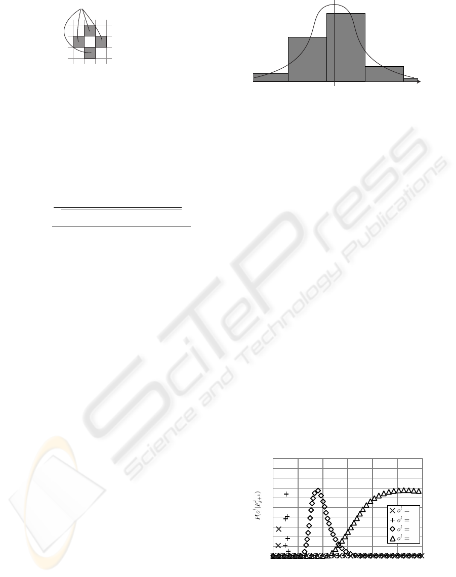
True disparity
pixel
Figure 6: Probability density of the observation of the dis-
parity.
3 EXPERIMENTS
3.1 Sensor Kernel Model of Stereo
Vision
We compared a map building result for the simula-
tion on a viewing ray and a real indoor scene using
our method and a conventional method considering
no sensor visibility nor spatial continuity.
In these experiments, we used edge-based stereo
vision for observation of obstacles. Stereo vision pro-
vides depth information for each edge feature and it
is well-known that the measurement error is inversely
proportional to square of the depth. In addition er-
roneous feature matching can be found in a certain
probability. Thus its sensor kernel model P(o
l
|F
l
k
),
required in Eqs.(4)- (7), are defined here as follows:
P(o
l
|F
l
k
) = P(T)P(o
l
|F
l
k
, T) + P(
¯
T)P(o
l
|F
l
k
,
¯
T) (21)
where o
l
is the measured disparity for the viewing
ray l, P(T) (fixed to 0.8 in the following experiment,
P(T)+P(
¯
T ≡ 1)) is the probability of obtaining a cor-
rect matching, P(o
l
|F
l
k
, T) is a gaussian (see Figure
6), P(o
l
|F
l
k
,
¯
T) is a uniform distribution over dispar-
ity range [0,60]. The obtained sensor kernel model
P(o
l
|F
l
k
) is shown in Figure 7.
0 50 200150100 250
25
10
3
1
0
1
0.5
distance[grid]
Figure 7: Observation model.
Our method updates the posteriors based on the
likelihoods considering sensor visibility, Eqs.(4)-(7).
PROBABILISTIC MAP BUILDING CONSIDERING SENSOR VISIBILITY
203
In the conventional method, we assume that state
of each grid is independent from state of other grid
as:
P(e
l
i
|o, O) =
P(o
l
i
|e
l
i
, O)P(e
l
i
|O)
P(o
l
i
|E
l
i
, O)P(E
l
i
|O) + P(o
l
i
|
¯
E
l
i
, O)P(
¯
E
l
i
|O)
(22)
where o
l
i
denotes the observation on ith grid and on
lth ray. On this assumption we can calculate each
grid indipendently. The following conventional like-
lihoods (Miura et al., 2002; Thrun, 2002a; Moravec,
1988) are adopted as a benchmark:
P(o
l
k
= o
E
|E
l
k
) = P(o
l
|F
l
k
) (23)
P(o
l
k
= o
E
|
¯
E
l
k
) = P(
¯
T) (24)
P(o
l
k
= o
¯
E
|E
l
k
) = P(
¯
T) (25)
P(o
l
k
= o
¯
E
|
¯
E
l
k
) = P(T){1− P(o
l
|F
l
k
, T)}. (26)
3.2 Posterior Update on a Viewing Ray
Our method of posterior update, of course, requires
an initial prior distribution. In addition it requires
an initial correlation parameter using for estimating
the spatial continuity. In the following experiment,
the initial prior P(E
i
) is uniformly set to 0.1 and the
spatial correlation c
q,q+1
to 0.871 where the grid size
is 5cm × 5cm These initial parameters are estimated
based on average obstacle size ( 40cm × 40cm ) in
actual room scene samples.
Since the aim of this paper is to show the effec-
tiveness of our posterior updating considering sensor
visibility, we suppose that the exact robot position and
orientation is known (NOT SLAM problem).
We compare our method with the convensional
one without considering sensor visibility. We use
three situations for the map update.
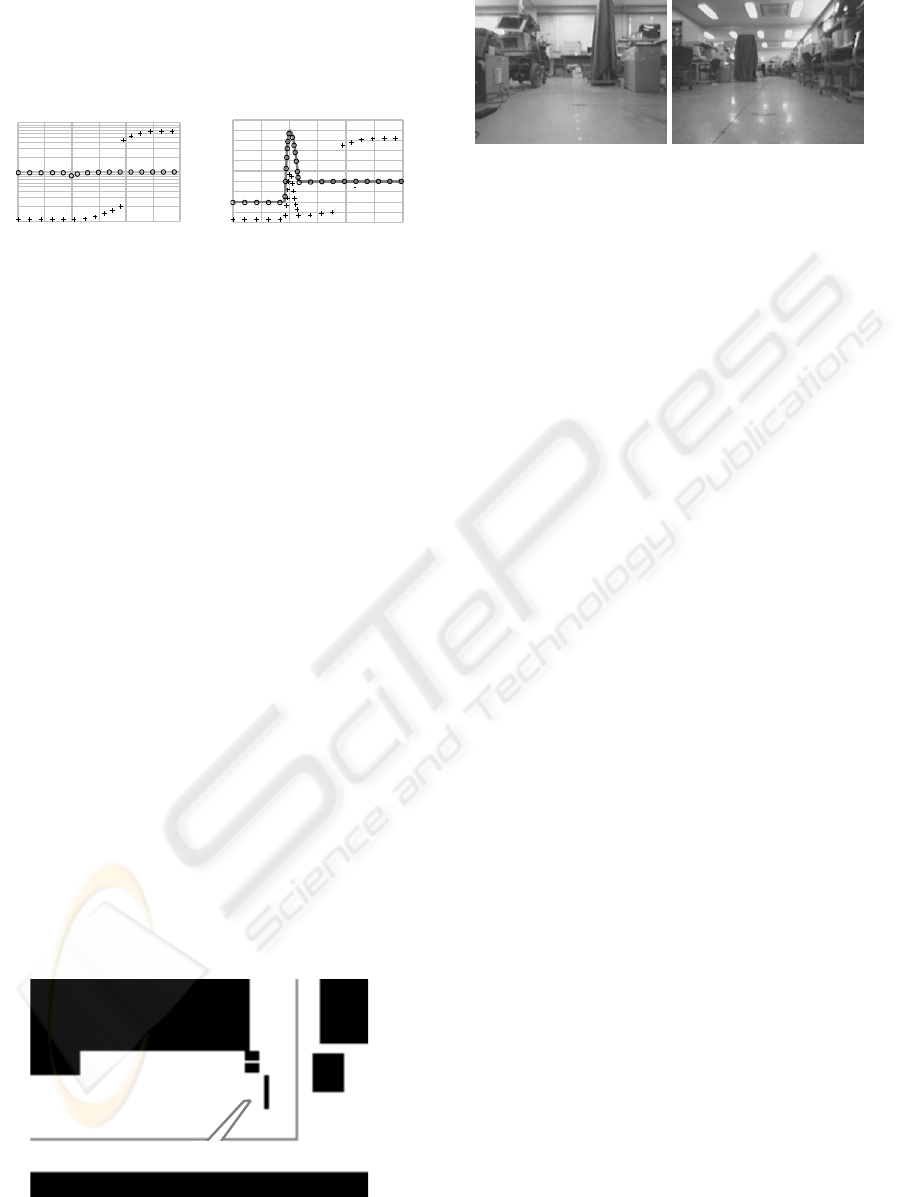
3.2.1 Case of Prior Probability of Uniform
Distribution
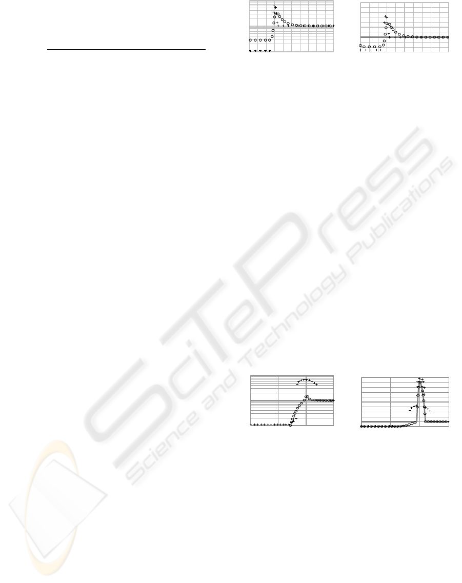
Figure 8 shows the likelihood ratio and the posteriors
when we take the observation ( equivalent to the dis-
parity of 10 pixels ) in the uniform disribution. With
considering sensor visibility, posteriors in the grid just
behind the 30th grid is higher than that without con-
sidering visibility because we consider the average
size of obstacles( equivalent to 40cm ) in this experi-
ment (see section 3.1).
3.2.2 Case of Uncertain Observation from
Distant Place
In Figure 9 we establish that posteriors are estimated
high from the 95th to the 110th grids after we obtain
0
50
100
1
0.1
10
likelihood ratio
distance[grid]
(a) Likelihood
50
0.5
0
1
distance[grid]
0
probability
100
(b) Result of posterior update
Figure 8: Result of posterior update when the robot get
the observation of the obstacle in the uniformly-distributed
probablity area. ”+” represents results of the conventional
method. ”” represents results of our method. The gray
curve in (b) represents the prior probablity.
the observations. Figure 9 shows the likelihood and
the posteriors when we get the observation ( equiva-
lent to the disparity of 3 pixels) with large error. With-
out considering visibility, posteriors in the range from
the 80th to the 120th grid ( equivalent to the dispar-
ity uncertainty of 3 pixels ) becomes high. But we
can not obtain the information in the range from the
90th to the 120th grid because we obtain the observa-
tion with the error which is larger than distribution of
obstacles. For this reason with considering visibility,
posteriors in the range from the 90th to the 120th grid
does not change as Figure 9(b). On the other hand,
in front of the range we can obtain the information
that the obstacles does not exist. For this reason both
methods show that posterior probability of obstacles
existence becomes low in front of the range.
0
50
100
1
0.1
10
150
likelihood ratio
distance[grid]
(a) Likelihood
50
100
0.5
0
1
probability
distance[grid]
0
150
(b) Result of posterior update
Figure 9: Result of posterior update when the robot get
the observation of the obstacle in the uniformly-distributed
probablity area. ”+” represents results of the conventional
method. ”” represents results of our method. The gray
curve in (b) represents the prior probablity.
3.2.3 Case of Failure Observation for Occluded
Area
In Figure 10 we establish that we obtain the failure
observation for an occluded area when existence of
obstacle is obvious. The error of this observation is
about from the 200th to the 560th grid ( equivalent to
the disparity of 1 pixel ). But it is highly possible that
ICINCO 2007 - International Conference on Informatics in Control, Automation and Robotics
204
the observation is failure because obstacle existence
about the 100th grid is already know. With consid-
ering sensor visibility, the failure observation is auto-
matically detected and the posteriors kept unchanged.
0
100
200
1
0.1
10
300
likelihood ratio
distance[grid]
(a) Likelihood
100
0.5
0
1
probability
distance[grid]
200
0
300
(b) Result of posterior update
Figure 10: Result of posterior update when the robot get
the observation of the obstacle in the uniformly-distributed
probablity area. ”+” represents results of the conventional
method. ”” represents results of our method. The gray
curve in (b) represents the prior probablity.
3.3 Result of Map Building
Next we show the result of map building for an ac-
tual room as shown in Figure 11. The mobile robot
moved in the room observing obstacles with stereo
cameras, starting from A point in Figure 11 via B, C,
B, D through the grey line in the figure, and finally
arrived at B point.
Figure 12 shows a view captured by the left cam-
era. Figure 12(a) is a view from A point, and Fig-
ure 12(b) is another view from B point. We com-
pared the built map of our method (Figure 14) to that
of the conventional one (Figure 13). Sub-figure (a)
and (b) of each figure shows the temporary map when
the robot reached to B point via A, B, C and D point
via A, B, C, B respectively, and sub-figure (c) shows
the final map after the robot arrived at B point. Our
method and the conventional method show the sig-
nificantly difference at the circular region labelled X.
The conventional method once estimate X as ’free-
space’ clearly when the robot was close to X (Figure
A
B
C
D
Figure 11: Rough map of obstacles.
(a) From A in Figure 11 (b) From D in Figure 11
Figure 12: Robot’s view.
13(a)). When the robot re-observedX region from far-
ther point, however, the detail information of X was
missing and estimated as ’obstacle’ rather than free-
space due to the erroneous stereo observation from far
point. (Figure 13(b),(c)). In contrast, our method cor-
rectly estimated the free-space in X without compro-
mise due to the erroneous observation from far point
(Figure 14(a),(b),(c)).
The process time for one update was about
1800ms on a PC with Athlon X2 4400+ CPU and
2GB memories.
4 CONCLUSIONS
We introduced a probabilistic observation model
properly considering the sensor visibility. Based on
estimating probabilistic visibility of each grid from
the current viewpoint, likelihoods considering sensor
visibility are estimated and then the posteriors of each
map grid are updated by Bayesian update rule. For
estimating grid visibility, Markov chain calculation
based on spatial continuity is employed based on the
knowledge of the average sizes of obstacles and free
areas.
This paper concentrates the aim on showing the
proof of concept of the probabilistic update consid-
ering sensor visibility and spatial continuity. For ap-
plication to the real robot navigation, SLAM frame-
work is necessary. In addition there are moving ob-
jects like human and semi-static objects like chairs
or doors in the real indoor scene. The expansion to
SLAM and environments with movable objects is the
future works.
PROBABILISTIC MAP BUILDING CONSIDERING SENSOR VISIBILITY
205
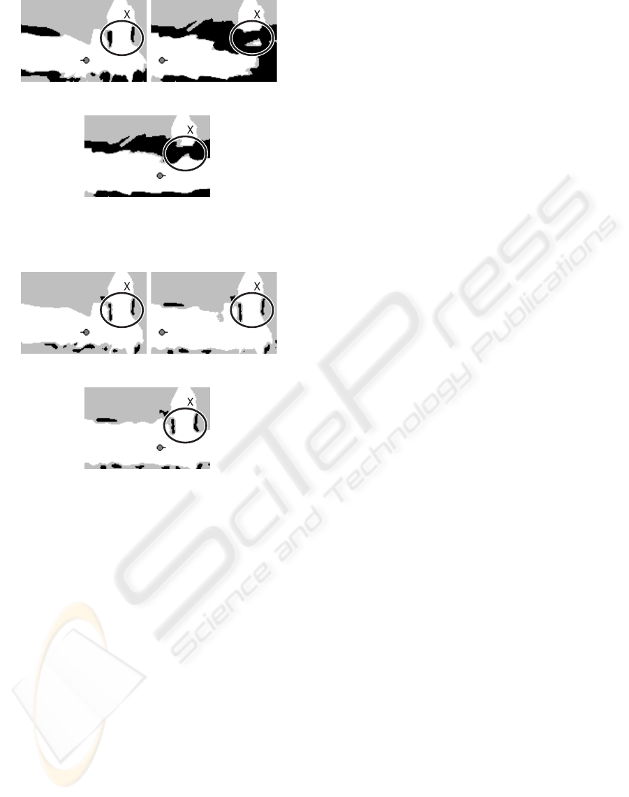
(a) At B via A, B, C (b) At D via A, B, C, B
(c) At B via A, B, C, B,
D
Figure 13: Result of map update without considering visibility
and spatial dependencies.
(a) At B via A, B, C (b) At D via A, B, C, B
(c) At B via A, B, C, B,
D
Figure 14: Result of map update considering visibility and spa-
tial dependencies.
REFERENCES
Grisetti, G., Stachniss, C., and Burgard, W. (2005). Improv-
ing Grid-based SLAM with Rao-Blackwellized Parti-
cle Filters by Adaptive Proposals and Selective Re-
sampling. In Proc. of the IEEE International Con-
ference on Robotics and Automation (ICRA), pages
2443–2448.
Miura, J., Negishi, Y., and Shirai, Y. (2002). Mobile
Robot Map Generation by Integrationg Omnidirec-
tional Stereo and Laser Range Finder. In Proc. of the
IEEE/RSJ Int. Conf. on Intelligent Robots and Systems
(IROS), pages 250–255.
Montemerlo, M. and Thrun, S. (2002). FastSLAM 2.0:
An Improved Particle Filtering Algorithm for Simul-
taneous Localization and Mapping that Provably Con-
verges.
Moravec, H. P. (1988). Sensor fusion in certainty grids for
mobile robots. In AI Magazine, Summer, pages 61–74.
Rachlin, Y., Dolan, J., and Khosla, P. (2005). Efficient map-
ping through exploitation of spatial dependencies. In
Proc. of the IEEE/RSJ Int. Conf. on Intelligent Robots
and Systems (IROS), pages 3117–3122.
Suppes, A., Suhling, F., and H
¨
otter, M. (2001). Robust Ob-
stacle Detection from Stereoscopic Image Sequences
Using Kalman Filtering. In DAGM-Symposium, pages
385–391.
Thrun, S. (2002a). Learning occupancy grids with forward
sensor models. In Autonomous Robots.
Thrun, S. (2002b). Robotic Mapping: A Survey. In Lake-
meyer, G. and Nebel, B., editors, Exploring Artifi-
cial Intelligence in the New Millenium. Morgan Kauf-
mann.
Thrun, S., Montemerlo, M., Koller, D., Wegbreit, B., Nieto,
J., and Nebot, E. (2004). FastSLAM: An Efficient So-
lution to the Simultaneous Localization And Mapping
Problem with Unknown Data Association. Journal of
Machine Learning Research.
ICINCO 2007 - International Conference on Informatics in Control, Automation and Robotics
206
