TIME-FREQUENCY REPRESENTATION OF INSTANTANEOUS
FREQUENCY USING A KALMAN FILTER
Jindřich Liška and Eduard Janeček
Department of Cybernetics, University of West Bohemia in Pilsen, Univerzitní 8, Plzeň, Czech Republic
Keywords: Instantaneous frequency, Kalman filter, time-frequency analysis, state estimation, Hilbert transform.
Abstract: In this paper, a new method for obtaining a time-frequency representation of instantaneous frequency is
introduced. A Kalman filter serves for dissociation of signal into modes with well defined instantaneous
frequency. A second order resonator model is used as a model of signal components – ‘monocomponent
functions’. Simultaneously, the Kalman filter estimates the time-varying signal components in a complex
form. The initial parameters for Kalman filter are obtained from the estimation of the spectral density
through the Burg’s algorithm by fitting an auto-regressive prediction model to the signal. To illustrate the
performance of the proposed method, experimental results show the contribution of this method to improve
the time-frequency resolution.
1 INTRODUCTION
Data analysis is a necessary part in pure research and
in practical applications. The problem of estimating
of a signal is of great interest in many areas of
engineering, such as energy processing, speech
recognition, vibration analysis and time series
modeling. To analyze a non-stationary data,
previous methods repeatedly apply block data
processing such as the short-time Fourier transform,
with the assumption, that the frequency
characteristics are time-invariant (or that the process
is stationary) for the duration of the time block. The
resolution of such methods is limited by the
Heisenberg-Gabor uncertainty principle.
In this work a different approach is proposed, in
which a Kalman filter is used to decompose the
time-varying signal into analytic components. As is
well known, the Kalman-filter can estimate the state
vectors of time-varying systems with knowledge of
the stochastic characteristics of the measurement
noise. The estimated components are then used for
computation of instantaneous amplitude and
frequency.
The rest of the paper is organized as follows. In
Section 2, a summary of the common non-stationary
data processing methods is presented. In Section 3,
we mention the instantaneous frequency
phenomenon. In Section 4, the use of Kalman filter
to obtain complex signal component estimation is
described. In Section 5, the results from experiments
and from real application are discussed. Conclusions
are drawn in Section 6.
2 NON-STATIONARY DATA
PROCESSING METHODS
The spectrogram is the most basic method, which is
a limited time window-width Fourier spectral
analysis. Since it relies on the traditional Fourier
transform, one has to assume the data to be
piecewise stationary. There are also practical
difficulties in applying the method: in order to
localize an event in time, the window width must be
narrow, but, on the other hand, the frequency
resolution requires longer time series (uncertainty
principle).
The wavelet approach is essentially a Fourier
spectral analysis with an adjustable window. For
specific applications, the basic wavelet function can
be modified according to special needs, but the form
has to be given before the analysis. In most common
applications, the Morlet wavelet is defined as
Gaussian enveloped sine and cosine wave groups
with 5.5 waves. It is very useful in analysing data
with gradual frequency changes. Difficulty of the
wavelet analysis is among others its non-adaptive
nature. Once the basic wavelet is selected then is
used to analyse all the data.
40
Liška J. and Jane
ˇ
cek E. (2007).
TIME-FREQUENCY REPRESENTATION OF INSTANTANEOUS FREQUENCY USING A KALMAN FILTER.
In Proceedings of the Fourth International Conference on Informatics in Control, Automation and Robotics, pages 40-46
DOI: 10.5220/0001621900400046
Copyright
c
 SciTePress

The Wigner-Ville distribution is sometimes also
referred to as the Heisenberg wavelet. By definition
it is the Fourier transform of the central covariance
function.
Above mentioned methods were used in Section
5 to compare their results with the output of the
method based on Kalman estimation.
3 INSTANTANEOUS
FREQUENCY AND THE
COMPLEX SIGNAL
Instantaneous frequency, )(t
ω
, is often defined as
derivation of phase
)(2
)(
)( tf
d
t
td
t
π
ϕ
ω ==
(1)
One of the ways how the unknown phase can be
obtained is to introduce a complex signal
)(tz
which corresponds to the real signal. As mentioned
in (Hahn, 1996) or in (Huang, 1998), the Hilbert
transform can be the elegant solution of this
problem.
The Hilbert transform,
)(tv , of a real signal
)(tu of the continuous variable
t
is
∫
∞
∞−
−
=
η
η
η
π
d
t
u
Ptv
)(1
)(
(2)
where
P
indicates the Cauchy Principle Value
integral. The complex signal
)(tz
)(
)()()()(
tj
etatvjtutz
ϕ
=⋅+=
(3)
whose imaginary part is the Hilbert transform
)(tv
of the real part
)(tu is then called the analytical
signal and its spectrum is composed only of the
positive frequencies of the real signal
)(tu .
From the complex signal, an instantaneous
frequency and amplitude can be obtained for every
value of
t
. Following (Hahn, 1996) the
instantaneous amplitude is defined as
22
)()()( tvtuta +=
(4)
and the instantaneous phase can be defined as
)(
)(
arctan)(
tu
tv
t =
ϕ
(5)
The instantaneous frequency then simplifies to
22
)()(
)()()()(
)
)(
)(
(arctan)(
tvtu
tutvtvtu
tu
tv
dt
d
t
+
−
==

ω
(6)
Even with the Hilbert transform, there is still
considerable controversy in defining the
instantaneous frequency as in (Boashash, 1992a).
Applying the Hilbert transform directly to a
multicomponent signal provides values of
)(ta and
)(t
ω
which are unusable for describing the signal.
The idea of instantaneous frequency and amplitude
does not make sense when a signal consists of
multiple components at different frequencies. This
leads Cohen in (Cohen, 1995)to introduce term
’monocomponent function’ where at any given time,
there is only one frequency value. Huang (Huang,
1998) introduced a so called Empirical Mode
Decomposition method to decompose the signal into
monocomponent functions (Intrinsic Mode
Functions).
4 USE OF KALMAN FILTER TO
OBTAIN THE SIGNAL
COMPONENTS
In this paper, an adaptive Kalman filter based
approach is used to decompose the analyzed signal
into monocomponent functions. As mentioned
above, it is required that the estimated components
are complex functions because of efficient
computation of the instantaneous frequency. The
analyzed signal is modeled as a sum of resonators in
this study.
4.1 Complex Signal Component Model
The second-order model ( 2=n ) of auto-regressive
(AR), linear time-invariant (LTI) system is
considered as a resonator. Its external description in
continuous domain is defined by the following
differential equation
)sin()( taty ⋅
⋅
=
ω
(7)
)cos()( taty ⋅
⋅
⋅
=
ω
ω

(8)
)()sin()(
22
tytaty ⋅−=⋅⋅−= ωωω

(9)
where a is the amplitude and
ω
is the natural
frequency of the resonator. Let the measured system
is described by its state equations:
TIME-FREQUENCY REPRESENTATION OF INSTANTANEOUS FREQUENCY USING A KALMAN FILTER
41

)()( txAtx
⋅
=

(10)
)()( txCty
⋅
=
(11)
where
)(tx denotes the vector of system internal
states (
)(tu and )(tv ) at time t, )(ty is the output
signal,
A
is the state matrix and C is the output
matrix. Hence it follows that the internal model
representation of the resonator with suitable selected
state variables (
)sin()( ttu ⋅=
ω
and )cos()( ttv
⋅
=
ω
)
is then
⎥
⎦
⎤
⎢
⎣
⎡
⋅
⎥
⎦
⎤
⎢
⎣
⎡
−
=
⎥
⎦
⎤
⎢
⎣
⎡
)(
)(
0
0
)(
)(
tv
tu
tv
tu
ω
ω


(12)
[]
⎥
⎦
⎤
⎢
⎣
⎡
⋅=
)(
)(
01)(
tv
tu
ty
.
(13)
The state equation (12) shows the state matrix of the
continuous model as a 2D rotation matrix whose
eigenvalues are pure imaginary numbers. The
trajectory in state space of such a system is a circle.
There is need to discretize the continuous state space
model for a digital computation needs. This can be
done by solving the state differential equation (14)
and substitution of the time
t
with sampling step
h (see Fairman, 1998)
)0()( xetx
At
= .
(14)
The discretized state model (
ht =Δ ) with state noise
)(k
ξ
and output noise )(k
η
is then
)(
)(
)(
)cos()sin(
)sin()cos(
)1(
)1(
k
kv
ku
hh
hh
kv
ku
ξ
ωω
ωω
⋅Γ+
⎥
⎦
⎤
⎢
⎣
⎡
⋅
⋅
⎥
⎦
⎤
⎢
⎣
⎡
⋅⋅
⋅−⋅
=
⎥
⎦
⎤
⎢
⎣
⎡
+
+
(15)
[] )(
)(
)(
01)( k
kv
ku
ky η ⋅Δ+
⎥
⎦
⎤
⎢
⎣
⎡
⋅=
(16)
The variables
)(k
ξ
and )(k
η
are white noise
vectors with identity covariance matrices. The
specific features of the noises are characterized by
the covariance matrices
Γ and Δ .
This resonator model forms together with Kalman
filtering approach an estimator of complex signal.
The estimation of the first model state is a real part
(sine function) and the estimation of the second
model state is an imaginary part (cosine function) of
the complex signal.
4.2 Discrete Kalman Filter
A discrete-time Kalman filter realizes a statistical
estimation of the internal states of noisy linear
system and it is able to reject uncorrelated
measurement noise – a property shared by all
Kalman filters. Let’s assume a system with more
components. Then the state matrix consists of
following blocks:
⎥
⎦
⎤
⎢
⎣
⎡
⋅⋅−
⋅⋅
=
)cos()sin(
)sin()cos(
ii
ii
i
hh
hh
A
ωω
ωω
(17)
and the state noise matrix blocks may be defined as
a derivative of the state matrix blocks:
⎥
⎦
⎤
⎢
⎣
⎡
⋅−⋅−
⋅⋅−
=
=
⋅∂
∂
=Γ
)sin()cos(
)cos()sin(
)(
ii
ii
i
i
i
hh
hh
h
A
ωω
ωω
ω
(18)
The derivation of state matrix blocks as an
estimation of the state noise matrix was selected
experimentally, because the derivation produces
blocks also in the state noise matrix and the
components relate to each other in the same manner
as in the state matrix.
The state-variable representation of the whole
system, which is characterized by the sum of
resonators, is given by the following matrices:
[]
.00
;
0000
00
00
0000
0000
;]010101[
;
000
0
00
000
000
)12(1
)12(2
2
1
21
22
2
1

…

…


…
…

…

…


…
…
+×
+×
×
×
=Δ
⎥
⎥
⎥
⎥
⎥
⎥
⎦
⎤
⎢
⎢
⎢
⎢
⎢
⎢
⎣
⎡
Γ
Γ
Γ
=Γ
=
⎥
⎥
⎥
⎥
⎥
⎥
⎦
⎤
⎢
⎢
⎢
⎢
⎢
⎢
⎣
⎡
=
n
nn
n
n
nn
n
C
A
A
A
A
δ
(19)
ICINCO 2007 - International Conference on Informatics in Control, Automation and Robotics
42

Commonly, the Kalman estimation includes two
steps – prediction and correction phase. Let’s
assume that the state estimate μ
0
is known with an
error variance P
0
. An a priori value of the state at
instant k+1 can be obtained as
kk
A
μ
μ
⋅
=
+1
(20)
The measured value
)(ky is then used to update the
state at instant k. The additive correction of the a
priori estimated state at k+1 is according to
(Vaseghi, 1987) proportional to the difference
between the a priori output at instant k defined as
⋅C μ
k
and the measured )(ky :
))((
1 kkkkk
CyKA
μ
μ
μ
⋅−
⋅
+⋅=
+
(21)
where
k
K is the Kalman gain which guarantees the
minimal variance of the error x
k
–μ
k
.
Also, at each step the variance
)1( +kP of the
error of μ
k+1
is calculated (see (Vaseghi, 1987)):
)(
1
TT
kk
TT
kk
ACPKAAPP ΔΓ+⋅−ΓΓ+=
+
(
22)
It is used for calculation of Kalman gain in the next
step of the recursive calculation (correction phase):
1
)()(
−
ΔΔ+⋅ΓΔ+=
TT
k
TT
kk
CCPCAPK
(23)
4.3 Estimation of Initial Parameters
The initial parameters for Kalman filter are obtained
from the estimation of the spectral density by fitting
an AR prediction model to the signal. The used
estimation algorithm is known as Burg’s method
(Marple, 1987), which fits an AR linear prediction
filter model of a specified order to the input signal
by minimizing the arithmetic mean of the forward
and backward prediction errors. The spectral density
is then computed from the frequency response of the
prediction filter. The AR filter parameters are
constrained to satisfy the Levinson-Durbin
recursion.
The initial Kalman filter parameters (frequencies
of the resonators) are then obtained as local maxima
of estimated spectral density which are greater than
a predefined level. These values indicate significant
frequencies in spectral density and determine the
order of the model (see Section 3.2).
5 RESULTS
Within this work three test signals are analyzed. The
first test signal s
1
(t) contains three harmonic
components.
kHz1
sampling rate was used and the
signal was 1 second long (
1000=N points). Signal
was formed by sinus functions with oscillation
frequencies f
1
=10Hz, f
2
=30Hz and f
3
=50Hz. The
amplitude was for all three components set to 10, but
the second component was zero for the first 0.5
seconds. The output noise with mean
0=m and
variance
1
=
σ
was added to the simulation signal.
The initial parameters for Kalman filter were
obtained through Burg’s AR linear prediction filter
of order 10 and the level for local maxima was
determined as
1max > . Under these conditions the
initial frequencies (n=3) for Kalman estimator were
obtained from Burg’s spectral density. The initial
conditions of Kalman estimator were set up in the
following way: μ
0
=[1…1], P
0
=10
6
.I, 1=
δ
, where
dim(μ
0
)= n
×
1 and dim(P
0
)= nn 22 × .
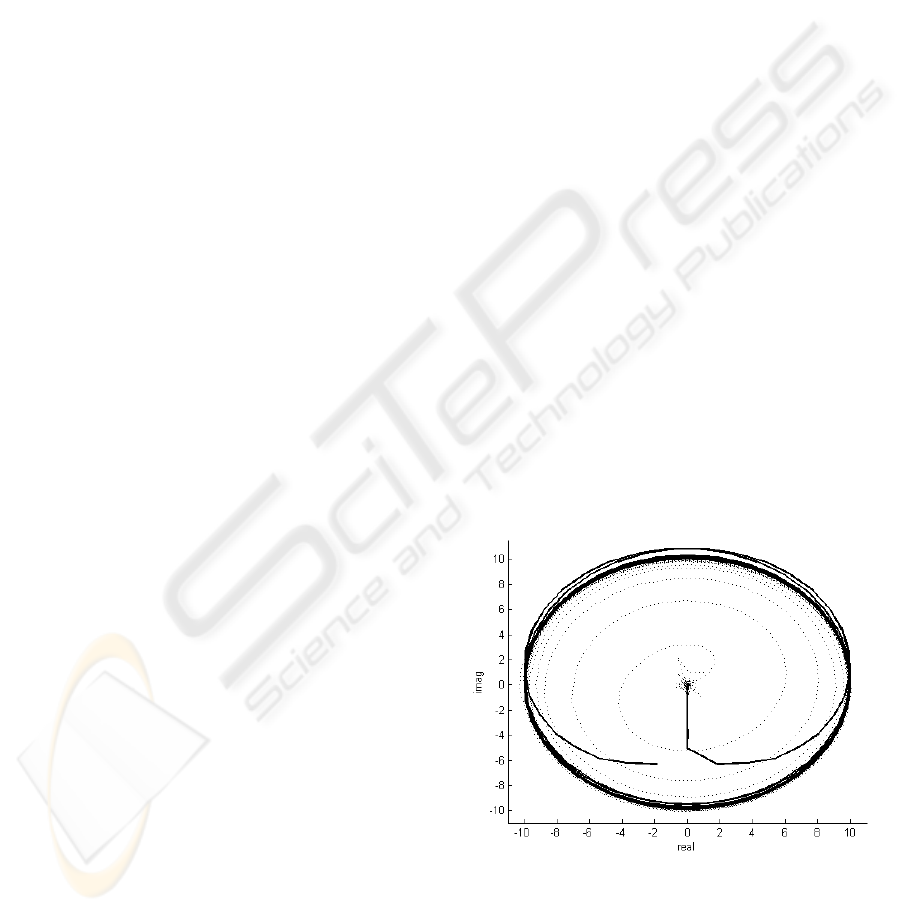
To take a look at the convergence of the
estimate, the comparison of the Hilbert approach and
Kalman filter is considered. In figure 1 the complex
signal of second component of the simulated signal
is displayed. The results were obtained through
Hilbert transform and through Kalman estimation.
The disadvantage of the Hilbert transform is that it
requires the pre-processing of the signal through
some signal decomposition method. To decompose
the signal into its components, the above introduced
algorithm uses the model of sum of resonators and
simultaneously the Kalman estimator is used to
estimate the time progression of these components.
Figure 1: Second component of test signal s
1
(t) - complex
signal obtained through Hilbert transform (solid line) and
through Kalman estimation (dotted line).
In figure 2, there is shown the instantaneous
frequency of all components of test signal s
1
(t).
TIME-FREQUENCY REPRESENTATION OF INSTANTANEOUS FREQUENCY USING A KALMAN FILTER
43

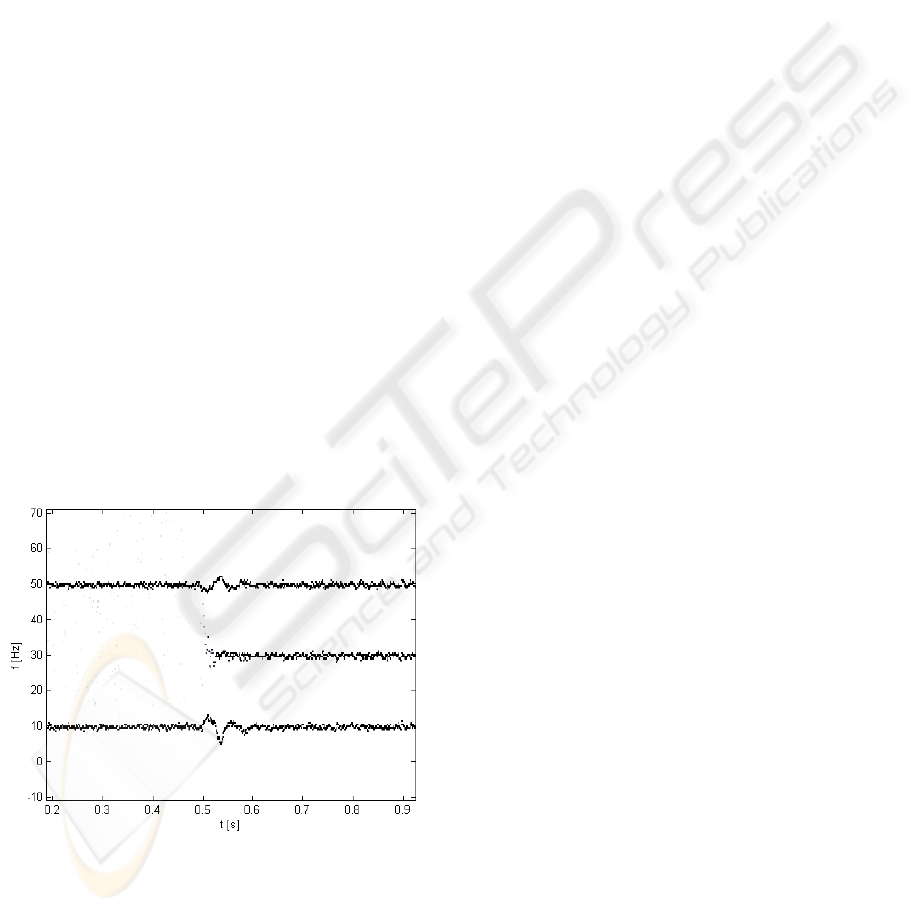
The additive noise in simulation signal is the cause
of the instantaneous frequency oscillating.
The algorithm based on Kalman estimation is
also illustrated on another two non-stationary test
signals s
2
(t) and s
3
(t). The initial conditions of
Kalman estimator were set up as mentioned above
and initial frequencies of the model were obtained
through Burg’s AR linear prediction filter of order
25 as maxima in estimated power spectrum (n=10).
The test signal s
2
(t) consists of two components
in time-frequency domain - stationary harmonic
signal with constant frequency and concave
parabolic chirp signal. Both components exist in
time between t = 100 and t = 900. The results of the
Kalman estimation is compared with the methods
mentioned in Section 2 and the results are shown in
Figure 4. The output of Kalman estimation in time-
frequency domain has relatively better time-
frequency resolution in both components than the
other methods.
The test signal s
3
(t) consists of four harmonic
components and the accuracy of the method to
identify the frequency and also the time of the origin
and end of the components is tested. The signal
begins again in time t = 100 and ends in t = 900. The
frequency changes in t = 300 and t = 600. There are
two components simultaneously in time between
t = 300 and t = 600. The ability of methods to
distinguish between these two frequencies is visible
in Figure 5. The smoothed pseudo Wigner-Ville
distribution and Kalman filter have better time-
frequency resolution compared to short-time Fourier
transform and to Morlet wavelet.
Figure 2: Estimation of instantaneous frequency of test
signal components.
The last example is the transform of the acoustic
signal from the real equipment where the
instantaneous event took place. The signal was
measured with 80 kHz sampling rate. For
comparison, in figure 3, the time-frequency-
amplitude responses of the short-time Fourier
transform (STFT) and of the Kalman estimator
approach are compared. The black column at first 4
milliseconds in the left spectrogram is the adaptation
phase of Kalman filter. This example was obtained
with following initial conditions: Burg’s filter of
order 400 was used to identify the power spectral
density and all local maxima (n=148), which satisfy
the inequality
>ma
x
10
-7
were appointed as
monitored frequencies. All resonance frequencies (5,
6, 14 and 27kHz) in the STFT spectrogram are also
presented in the left one (Kalman). An event which
occurs at time 0.022 seconds is displayed also in
both spectrograms (see the frequency band 2 -
15 kHz). It is visible that the Kalman version of
spectrogram offers a better resolution in time and
frequency than the spectrogram obtained through
STFT.
6 CONCLUSIONS
The new method for obtaining the time-frequency
representation of instantaneous frequency has been
introduced in this work. The procedure is based on
the Kalman estimation and shares its advantages
regarding the suppression of measurement noise. In
this method the Kalman filter serves for dissociation
of signal into modes with well defined instantaneous
frequency. Simultaneously the time progression of
signal components is estimated. This procedure
utilizes the adaptive feature of the Kalman filter.
In cases where the short–time Fourier transform
cannot offer sufficient resolution in frequency-time
domain, there can be taken advantage of this method
despite of higher computational severity. In
vibrodiagnostic methods, where frequency-time
information is used for localizing of non-stationary
events, the sharpness of the introduced method can
be helpful for the improvement of the event
localization.
ACKNOWLEDGEMENTS
This work was supported by AREVA NP GmbH,
Department SD-G in Erlangen (Germany) and from
the specific research of Department of Cybernetics
at the University of West Bohemia in Pilsen.
ICINCO 2007 - International Conference on Informatics in Control, Automation and Robotics
44

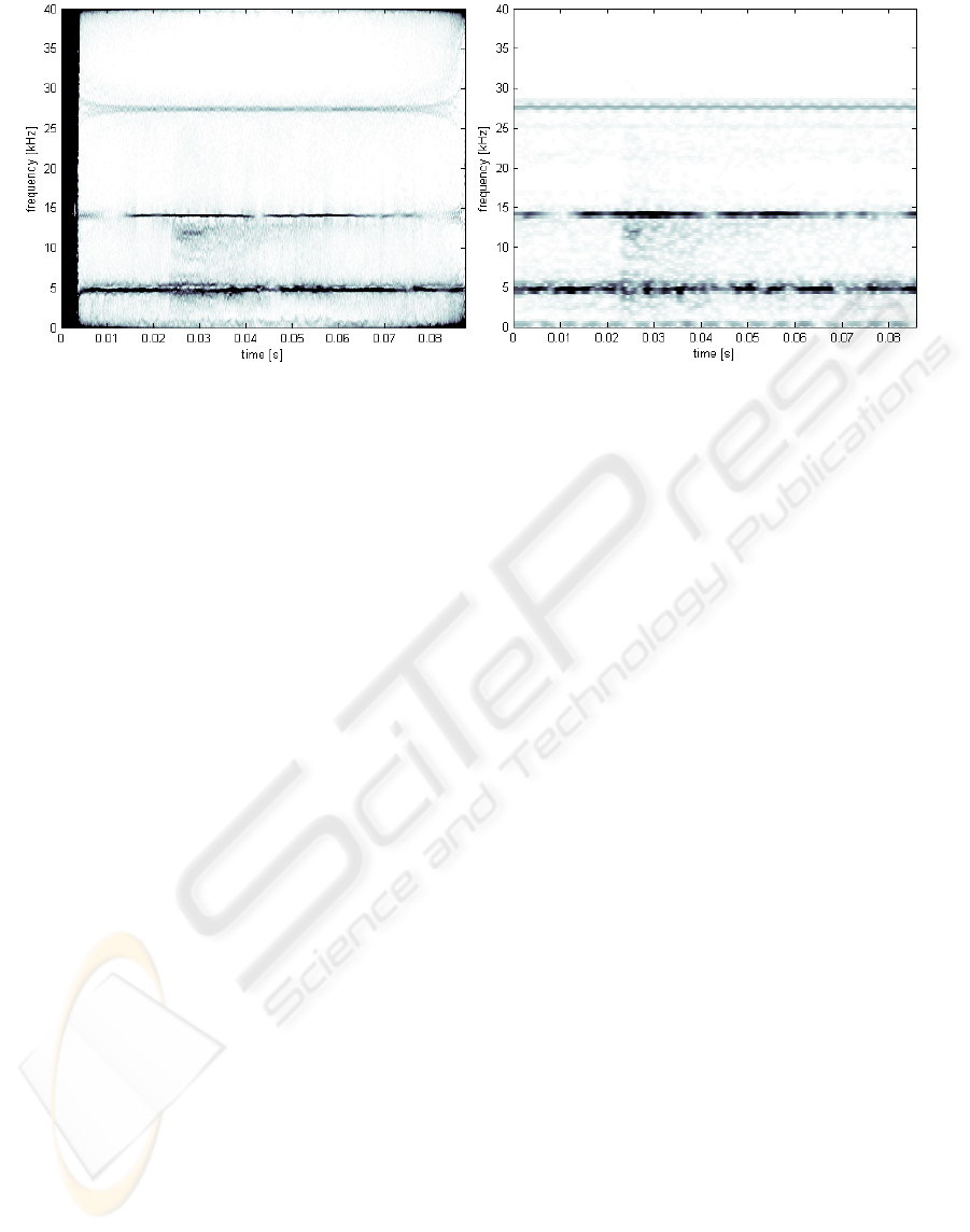
Figure 3: Spectrogram using Kalman estimation (left) and using short-time Fourier transform (right).
REFERENCES
Boashash, B., 1992a. Estimating and Interpreting the
Instantaneous Frequency of a Signal – Part 1:
Fundamentals. In Proceedings of the IEEE, vol. 80,
no. 4, pp. 520-538.
Boashash, B., 1992b. Estimating and Interpreting the
Instantaneous Frequency of a Signal – Part
2:Algorithms and Applications. In Proceedings of
the IEEE, vol. 80, no. 4, pp. 540-568.
Cohen, L., 1995. Time-Frequency Analysis, Prentice
Hall PTR. New Jersey.
Hahn, S.L., 1996. Hilbert Transforms in Signal
Processing, Artech House. Boston.
Huang, N.E., et al., 1998. The empirical mode
decomposition and the Hilbert spectrum for
nonlinear and non-stationary time series analysis. In
Proc.R.Soc.Lond. A, vol. 454, no. 1971, pp. 903-995.
Huang, N. E., 2003. A confidence limit for the empirical
mode decomposition and the Hilbert spectral
analysis. In Proc. Roy. Soc. Lond., 459, pp. 2317-
2345, 2003
Rilling, G., Flandrin, P., Goncalves, P., 2003. On
Empirical Mode Decomposition and its Algorithms.
In IEEE-EURASHIP workshop on nonlinear signal
an image processing NSIP-03
Maragos, P., Kaiser, J.F., Quantieri, T.F., 1993. On
Amplitude and Frequency Demodulation Using
Energy Operators. In IEEE Trans. on Signal
Processing, vol. 41, no. 4, pp. 1532-1550.
Marple, S.L., 1987. Digital Spectral Analysis, Prentice
Hall. New Jersey.
Vaseghi, S.V., 2000. Advanced Digital Signal
Processing and Noise Reduction, John Wiley &
Sons. New Jersey.
Fairman, F.W., 1998. Linear Control Theory: The State
Space Approach, John Wiley& Sons. Toronto
TIME-FREQUENCY REPRESENTATION OF INSTANTANEOUS FREQUENCY USING A KALMAN FILTER
45

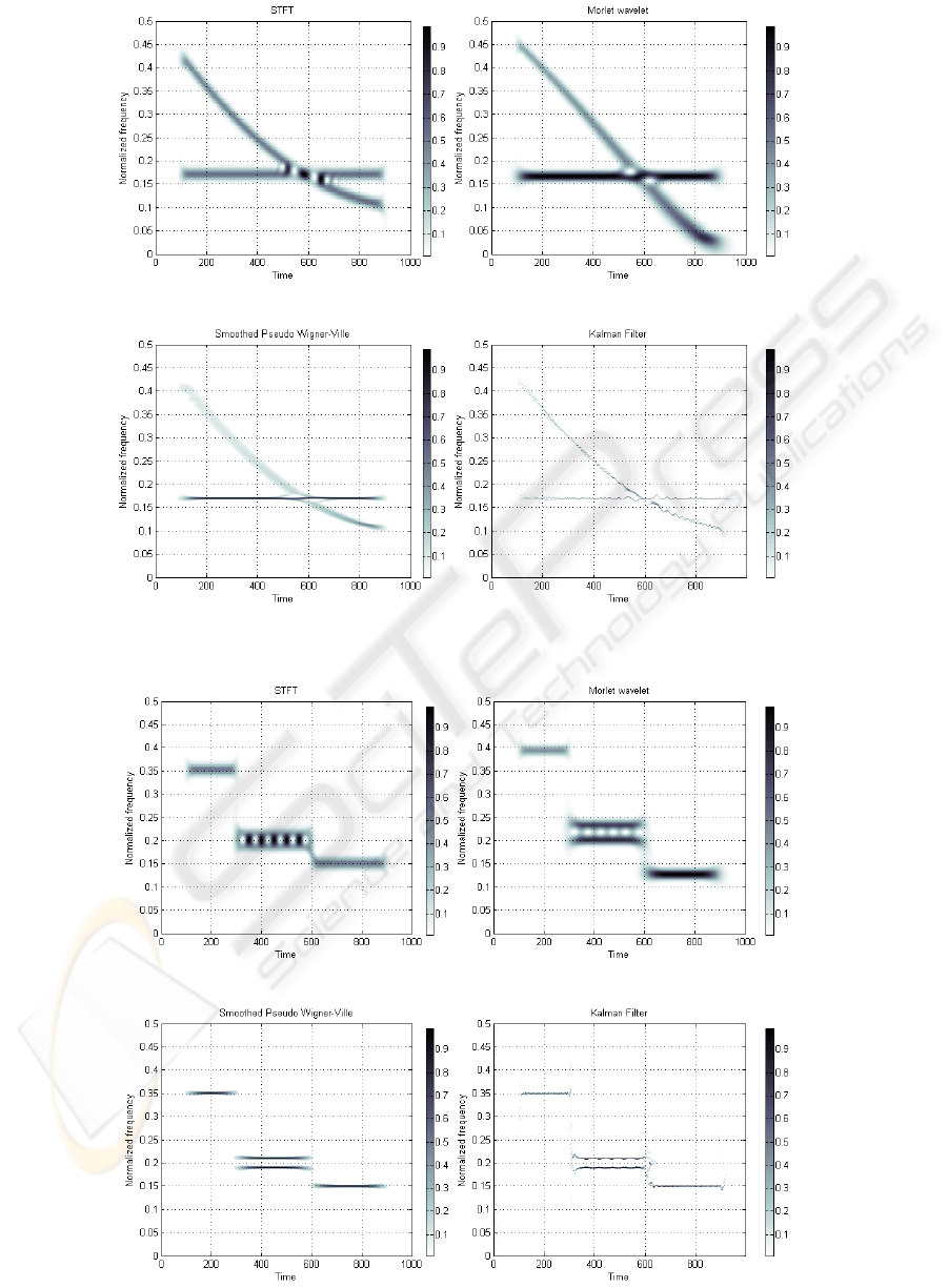
Figure 4: Time-frequency analysis results of the test signal s
2
(t).
Figure 5: Time-frequency analysis results of the test signal s
3
(t).
ICINCO 2007 - International Conference on Informatics in Control, Automation and Robotics
46