INCREMENTAL PROCESSING OF TEMPORAL OBSERVATIONS IN

SUPERVISION AND DIAGNOSIS OF DISCRETE-EVENT SYSTEMS

Gianfranco Lamperti

Dipartimento di Elettronica per l’Automazione

Via Branze 38, 25123 Brescia, Italy

Marina Zanella

Dipartimento di Elettronica per l’Automazione

Via Branze 38, 25123 Brescia, Italy

Keywords:

Diagnosis, supervision, discrete-event systems, temporal observations, indexing techniques, uncertainty.

Abstract:

Observations play a major role in supervision and diagnosis of discrete-event systems (DESs). In a distributed,

large-scale setting, the observation of a DES over a time interval is not perceived as a totally-ordered sequence

of observable labels but, rather, as a directed acyclic graph, under uncertainty conditions. Problem solving,

however, requires generating a surrogate of such a graph, the index space. Furthermore, the observation

hypothesized so far has to be integrated at the reception of a new fragment of observation. This translates

to the need for computing a new index space every time. Since such a computation is expensive, a naive

generation of the index space from scratch at the occurrence of each observation fragment becomes prohibitive

in real applications. To cope with this problem, the paper introduces an incremental technique for efﬁciently

modeling and indexing temporal observations of DESs.

1 INTRODUCTION

Observations are the inputs to several tasks that can

be carried out by exploiting Model-Based Reasoning

techniques. Typically, they are the inputs to super-

vision, control and monitoring of physical processes

(Roz

e, 1997); they represent the symptoms of diag-

nosis (Brusoni et al., 1998); they are the clues for

history reconstruction (Baroni et al., 1997; Baroni

et al., 1999), and the test cases for software debug-

ging (Wotawa, 202; K

ob and Wotawa, 2004) . Tem-

poral observations refer to dynamical systems and

processes, and are endowed not only with a logical

content, describing what has been observed, but also

with a temporal content, describing when it has been

observed.

Both (independent) aspects, can be mod-

eled either quantitatively or qualitatively. This paper

addresses the most qualitative abstraction of the no-

tion of a temporal observation, i.e. an observation

whose logical and temporal contents are both qualita-

tive. This abstraction is quite important since adopt-

ing qualitative models is an issue of Model-Based

Reasoning and Qualitative Physics as well, in far as

reasoning about (a ﬁnite number of) qualitative val-

Indeed, in several contexts, the time a value is observed

is not relevant, while it is interesting to know the time such

a value was generated by the considered system/process.

ues is easier and computationally cheaper. Moreover,

adopting a higher abstraction level ﬁrst, so as to focus

attention, and a more detailed level later, is a princi-

ple of hierarchical model-based diagnosis (Mozeti

1991). A general model for (qualitative uncertain)

temporal observations was proposed in (Lamperti and

Zanella, 2002), and exploited for describing the in-

put of an a posteriori diagnosis task. Such a model

consists of a directed acyclic graph where each node

contains an uncertain logical content and each edge is

a temporal precedence relationship. Thus, the graph,

altogether, shows all the uncertain values observed

over a time interval and their partial temporal order-

ing. Each uncertain logical content ranges over a set

of qualitative values (labels). Therefore the observa-

tion graph implicitly represents all the possible se-

quences of labels consistent with the received tem-

poral observation, where each sequence is a sentence

of a language. Then, the observation graph, although

intuitive and easy to build from the point of view of

the observer, is unsuitable for processing. For any fur-

ther processing it is better to represent a language in

the standard way regular languages are represented

(Aho et al., 1986), that is, by means of a determin-

istic automaton. In (Lamperti and Zanella, 2002)

this automaton is called index space and it is built

as the transformation of a nondeterministic automa-

Lamperti G. and Zanella M. (2006).

INCREMENTAL PROCESSING OF TEMPORAL OBSERVATIONS IN SUPERVISION AND DIAGNOSIS OF DISCRETE-EVENT SYSTEMS.

In Proceedings of the Eighth International Conference on Enterprise Information Systems - AIDSS, pages 47-57

DOI: 10.5220/0002447200470057

 SciTePress

Figure 1: Power transmission network.

ton drawn from the observation graph. The problem

arises when the nodes of the observation graph are re-

ceived one at a time, typically in supervision and di-

agnosis of dynamical systems, in particular, discrete-

event systems (DESs). In fact, the supervision process

is required to react at each occurring piece of obser-

vation so as to generate appropriate diagnostic infor-

mation (Lamperti and Zanella, 2004a; Lamperti and

Zanella, 2004b). This translates to the need for gener-

ating a new index space at each new reception. How-

ever, a naive approach, that each time makes up the

new index space from scratch, would be inadequate

from the computational point of view. We need there-

fore an incremental technique for index-space gener-

ation.

2 APPLICATION DOMAIN

We consider a reference application domain of power

networks. A power network is composed of trans-

mission lines. Each line is protected by two breakers

that are commanded by a protection. The protection

is designed to detect the occurrence of a short circuit

on the line based on the continuous measurement of

its impedance: when the impedance goes beyond a

given threshold, the two breakers are commanded to

open, thereby causing the extinction of the short cir-

cuit. In a simpliﬁed view, the network is represented

by a series of lines, each one associated with a pro-

tection, as displayed in Fig. 1, where lines l

···l

are protected by protections p

···p

, respectively.

For instance, p

controls l

by operating breakers b

and b

. In normal (correct) behavior, both breakers

are expected to open when tripped by the protection.

However, the protection system may exhibit an ab-

normal (faulty) behavior, for example, one breaker or

both may not open when required. In such a case,

each faulty breaker informs the protection about its

own misbehavior. Then, the protection sends a re-

quest of recovery actions to the neighboring protec-

tions, which will operate their own breakers appro-

priately. For example, if p

operates b

and b

and

the latter is faulty, then p

will send a signal to p

which is supposed to command b

. A recovery ac-

tion may be faulty on its turn. For example, b

may

not open when tripped by p

, thereby causing a fur-

ther propagation of the recovery to protection p

. The

protection system is designed to propagate the recov-

ery request until the tripped breaker opens correctly.

Figure 2: Genesis of a temporal observation.

When the protection system is reacting, a subset of

the occurring events are visible to the operator in a

control room who is in charge of monitoring the be-

havior of the network and, possibly, to issue explicit

commands so as to minimize the extent of the isolated

subnetwork. Typical visible events are short (a short

circuit occurred on the line), open (a breaker opened),

close (a breaker closed), and end (the short circuit ex-

tinguished). Generally speaking, however, the local-

ization of the short circuit and the identiﬁcation of the

faulty breakers may be impractical in real contexts,

especially when the extent of the isolation spans sev-

eral lines and the operator is required to take recovery

actions within stringent time constraints. On the one

hand, there is the problem of observability: the ob-

servable events generated during the reaction of the

protection system are generally incomplete and un-

certain in nature. On the other, whatever the observa-

tion, it is impractical for the operator to reason on the

observations so as to make consistent hypotheses on

the behavior of the system and, eventually, to estab-

lish the shorted line and the faulty breakers.

3 TEMPORAL OBSERVATIONS

A temporal observation O is the mode in which the

observable labels, generated by the evolution of a

DES, are perceived by the observer. Considering the

realm of asynchronous DESs, such as active systems

(Lamperti and Zanella, 2003), a history h of a sys-

tem is a sequence of component transitions, where

each transition refers to a communicating automa-

ton. Thus, h = T

,...,T

. Since a subset of

the transitions are visible, the system history is ex-

pected to generate a sequence of observable labels,

namely a temporal sequence 

,...,

, where each



, i ∈ [1 .. k], is the label generated by a visible tran-

sition in h. However, due to the multiplicity of com-

munication channels between the (distributed) system

and the observer, and to noise on such channels, the

temporal observation O received by the observer is

likely to differ from the temporal sequence generated

by the system (see Fig. 2). Intuitively, O is a se-

quence of temporal fragments bringing information

about what/when something is observed. Formally,

let Λ be a domain of observable labels, possibly in-

cluding the null label ε.

A temporal fragment ϕ is a

The null label ε is invisible to the observer.

ICEIS 2006 - ARTIFICIAL INTELLIGENCE AND DECISION SUPPORT SYSTEMS

pair (λ, τ), where λ ⊆ Λ is called the logical content,

and τ is a set of fragments, called the temporal con-

tent. Speciﬁcally, O is a sequence of temporal frag-

ments, O = ϕ

,...,ϕ

, such that

∀i ∈ [1 .. n],ϕ

=(λ

,τ

)(τ

⊆{ϕ

,...,ϕ

i−1

}) .

The temporal content of a fragment ϕ is supposed to

refer to a (possibly empty) subset of the fragments

preceding ϕ in O. Thus, a fragment is uncertain in

nature, both logically and temporally. Logical un-

certainty means that λ includes the actual (possibly

null) label generated by a system transition, but fur-

ther spurious labels may be involved too. Temporal

uncertainty means that only partial ordering is known

among fragments. As such, both logical and temporal

uncertainty are a sort of relaxation of the temporal se-

quence generated by the system, the former relaxing

the actual visible label into a set of candidate labels,

the latter relaxing absolute temporal ordering into par-

tial ordering.

A sub-observation O

[i]

of O, i ∈ [0 .. n], is the

(possibly empty) preﬁx of O up to the i-th fragment,

[i]

= ϕ

,...,ϕ

.

Example 1. Let Λ={short, open,ε}, O = ϕ

, ϕ

, where ϕ

=({short,ε}, ∅), ϕ

({open,ε}, {ϕ

}), ϕ

=({short, open}, {ϕ

}),

=({open}, {ϕ

}). ϕ

, is logically uncertain (ei-

ther short or nothing is observed). ϕ

follows ϕ

and

is logically uncertain (open vs. nothing). ϕ

follows

and is logically uncertain (short vs. open). ϕ

fol-

lows ϕ

and is logically certain (open). However, no

temporal relationship is deﬁned between ϕ

and ϕ

or ϕ

. 2

Based on Λ, a temporal observation O =

ϕ

,...,ϕ

 can be represented by a DAG, called an

observation graph,

γ(O)=(Λ, Ω, E)

where Ω={ω

,...,ω

} is the set of nodes isomor-

phic to the fragments in O, each node being marked

by a nonempty subset of Λ, and E is the set of edges

isomorphic to the temporal content of fragments in O:

∀ω

∈ Ω,ϕ

=(λ

,τ

),ϕ

∈ τ

→ N

∈ E),

∀(ω

→ ω

∈ E)(ϕ

∈ τ

,ϕ

=(λ

,τ

)).

A precedence relationship is deﬁned between nodes

of the graph, speciﬁcally, ω ≺ ω



means that γ(O)

includes a path from ω to ω



, while ω  ω



means

either ω ≺ ω



or ω = ω



Example 2. Consider the observation O deﬁned

in Example 1. The relevant observation graph

γ(O) is shown in Fig. 3. Note how γ(O) implic-

itly contains several candidate temporal sequences,

each candidate sequence generated by picking up

a label from each node of the graph without vi-

olating the partially-ordered temporal relationships

Figure 3: Observation graph γ(O).

among nodes. Possible candidates are, among oth-

ers, short, open, short, open, short, open, open,

and short , open.

However, we do not know which

of the candidates is the actual temporal sequence gen-

erated by the system, the other ones being the spu-

rious candidate sequences. Consequently, from the

observer viewpoint, all candidate sequences share the

same ontological status. 2

4 INDEXING OBSERVATIONS

The rationale of the paper is that, both for computa-

tional and space reasons, the observation graph is in-

convenient for carrying out a task that takes as input

a temporal observation. This claim applies to linear

observations as well, which are merely a sequence O

of observable labels. In this case, it is more appropri-

ate to represent each sub-observation O



⊆ O as an

integer index i corresponding to the length of O



.As

such, i is a surrogate of O



. The same approach have

been proposed for graph-based temporal observations

(Lamperti and Zanella, 2000). However, we need ex-

tending the notion of an index appropriately and make

model-based reasoning on a surrogate of the temporal

observation, called an index space.

Let γ(O)=(Λ, Ω, E) be an observation graph. A

preﬁx P of O is a (possibly empty) subset of Ω where

∀ ω ∈P( ω



∈P(ω



≺ ω)).

The formal deﬁnition of an index space is supported

by the introduction of two functions on P. The set of

consumed nodes up to P is

Cons(P)={ω | ω ∈ Ω,ω



∈P,ω  ω



}. (1)

The set of consumable nodes from P, called the fron-

tier of P, is deﬁned as

Front (P)={ω | ω ∈ (Ω − Cons(P)),

∀(ω



→ ω) ∈ E (ω



∈ Cons(P))}. (2)

The fact that the length of a candidate temporal se-

quence may be shorter than the number of nodes in the ob-

servation graph comes from the immateriality of the null

label ε, which is ‘transparent’. For instance, candidate

ε, ε, short , open is in fact short, open.

INCREMENTAL PROCESSING OF TEMPORAL OBSERVATIONS IN SUPERVISION AND DIAGNOSIS OF

DISCRETE-EVENT SYSTEMS

Example 3. Considering γ(O) in Fig. 3, with P =

{ω

,ω

},wehaveCons(P)={ω

,ω

} and

Front (P)={ω

}. 2

The two functions deﬁned on an index are formally

related to one another by Theorem 1.

Theorem 1. The frontier of an index  is empty iff the

set of consumable nodes of  equals the set of nodes

of the observation graph:

Front ()=∅⇐⇒Cons()=Ω. (3)

Proof (sketch). When Ω=∅ (empty observa-

tion), Eq. (3) is trivially proven. Thus, we assume

Ω = ∅. Considering Front ()=∅, based on Eq. (2),

we have {ω | ω ∈ (Ω − Cons()), ∀(ω



→ ω) ∈

E (ω



∈ Cons())} = ∅. Assume Cons() ⊂ Ω.

Let ¯ω ∈ (Ω − Cons()). Three scenarios are possi-

ble:

(a) ∀(ω



→ ¯ω) ∈ E (ω



∈ Cons()). In this case,

Eq. (2) is satisﬁed for ω =¯ω, that is, Front () =

∅, a contradiction.

(b) ω



(ω



→ ¯ω ∈ E). Even in this case, Eq. (2)

is satisﬁed for ω =¯ω, as the condition ∀(ω



→

ω) ∈ E (ω



∈ Cons()) is trivially true. Thus,

Front () = ∅, a contradiction.



→ ¯ω) ∈ E (ω



/∈ Cons()). This sce-

nario makes the universal predicate in Eq. (2) false.

However, we may choose a different node in (Ω −

Cons()), rather than ¯ω, speciﬁcally one of the ω



satisfying the existential predicate in scenario (c).

This way, the above three scenarios are possible

for the new node too. In particular, if either (a)

or (b) holds, Front () = ∅, a contradiction. If

cursively, until either (a) or (b) holds. Since the

observation graph is a DAG, such a recursion will

end at the either (a) or (b), that is, Front () = ∅,a

contradiction.

Thus, Front ()=∅ =⇒ Cons()=Ω. Con-

versely, assume Cons()=Ωand Front () = ∅.

Based on Eq. (2), Front () includes an ω in

(Ω − Cons()) = ∅, a contradiction. Thus,

Cons()=Ω =⇒ Front ()=∅.

Let O be a temporal observation. The preﬁx space

of O is the nondeterministic automaton

Psp(O)=(S

, L

, T

, S

)

where

= {P | P is a preﬁx of O}

is the set of states,

= { |  ∈ λ, (λ, τ) ∈ Ω}

is the set of labels,

= ∅

Figure 4: Preﬁx space Psp(O) and index space Isp(O),

where O is depicted in Fig. 3.

is the initial state,

= {P | P ∈ S

, Cons(P)=Ω}

is the set of ﬁnal states, and T

: S

× L

→ 2

is the transition function such that P



−→P



∈ T

iff,

deﬁning the ‘⊕’ operation as

P⊕ω =(P∪{ω}) −{ω



| ω



∈P,ω



≺ ω}, (4)

we have:

ω ∈ Front (P),ω =(λ, τ),∈ λ, P



= P⊕ω.

The index space of O is the deterministic automaton

Isp(O)=(S, L, T,S

, S

)

equivalent to Psp(O). Each state in Isp(O) is an in-

dex of O. The peculiarity of an index space is that

each path from S

to a ﬁnal state is a mode in which

we may choose a label in each node of the observation

graph γ(O) based on the partial ordering imposed by

γ(O) (Lamperti and Zanella, 2002).

Example 4. Consider γ(O) in Fig. 3. Shown in Fig. 4

are the preﬁx space Psp(O) (left) and the index space

Isp(O) (shaded). Each preﬁx is written as a string

of digits, e.g., 24 stands for P = {ω

,ω

}. Fi-

nal state are double circled. According to the stan-

dard algorithm that transforms a nondeterministic au-

tomaton to a deterministic one (Aho et al., 1986),

each node of Isp(O) is identiﬁed by a subset of the

nodes of Psp(O). Nodes in Isp(O) have been named



···

. These are the indexes of O. 2

As for observations, we may deﬁne a restriction of

the index space up to the i-th fragment as follows. Let

Isp(O)=(S, L, T,S

, S

) be an index space, where

γ(O)=(Λ, Ω, E), Ω={ω

,...,ω

}. Let S be a

node in S. The sub-node S

[i]

of S, i ∈ [0 .. n],is

[i]



if i =0

{ |  ∈ S, ∀ω

∈(j ≤ i)} otherwise.

(5)

The sub-index space Isp

[i]

of O, i ∈ [0 .. n],isan

automaton

Isp

[i]

(O)=(S



, L



, T



, S



)

ICEIS 2006 - ARTIFICIAL INTELLIGENCE AND DECISION SUPPORT SYSTEMS

where



= {S



| S ∈ S,S



= S

[i]



= ∅}



= {T



| T ∈ T,T = S



−→ S



= S



−→ S



= S

[i]



= ∅,S



= S

[i]



= ∅}



= { | S



−→ S



∈ T



}



= {S



| S



∈ S



, ∈S



Cons()={ω

,...,ω

}}.

The formal relationship between sub-observations

and sub-index spaces is stated by Theorem 2.

Theorem 2. The sub-index space of an observation

equals the index space of the sub-observation,

Isp

[i]

(O)=Isp(O

[i]

). (6)

Proof (sketch). The proof is supported by two lem-

mas. Lemma 2.1 is based on the relationship between

a nondeterministic automaton, A

, and its equivalent

deterministic one, A

, based on the subset construc-

tion (Aho et al., 1986). Closure(N

) denotes the clo-

sure of node N

in A

. This is the set made up by

and all the nodes that are reachable from N

via

ε-transitions in A

. Lemma 2.2 is grounded on the

deﬁnition of Psp(O) and, particularly, on Eq. (4).

Lemma 2.1. Let N



−→ N

be a transition in an index

space Isp(O). Then,

(i) There exists

⊆ N

= ∅, such that

∀ ∈

(



−→



∈ Psp(O), 



∈ N

Closure(



) ⊆ N

);

(ii) All 



∈ N

meet the condition stated in point (i).

Lemma 2.2. Let 



−→



be a transition in Psp(O).

Let Max () denote the most recent fragment of  in

O, Max ()=i | ω

∈, ∀ω

∈(j ≤ i). Then,

Max (



) ≥ Max ().

Theorem 2 can be proved by induction on the nodes

of the two automata in Eq. (6). The basis states the

equality of the initial states. Let S

and S



be the

initial states of Isp

[i]

(O) and Isp(O

[i]

), respectively.

Based on the lemmas above and Eq. (5), an index

∈S

belongs to the closure of the root of Psp(O)

and is only composed of nodes ω

such that j ≤ i.

Thus, ∈S



. Conversely, 



∈ S



belongs to the

closure of the root of Psp(O

[i]

) and is only composed

of nodes ω

such that j ≤ i, thereby 



∈ S

.In

other terms, S

= S



. Now we show the equality of

the transition functions.

Assume a transition N



−→ N

∈ Isp

[i]

(O), where

is also a node in Isp(O

[i]

). We show that the same

Figure 5: Psp(O

[3]

), Isp(O

[3]

), and Isp

[3]

(O).

transition is in Isp(O

[i]

) too. Since N

and N

are

the sub-nodes of two nodes in Isp(O), namely N

and N

, respectively, N

will not include the indexes





such that 



−→



∈ Psp(O), 



∈ Closure(



and either ∈(N

− N

) or ω

∈



where j>i.

Let 

∈ N

. As such, 

only includes indexes

where j ≤ i. Thus, 

is reachable in Psp(O)

from an index in N

via a path of transitions, the ﬁrst

being marked by  and the other ones by ε, each of

them relevant to a node ω

where j ≤ i. There-

fore, there exists a transition in Isp(O

[i]

) that is rooted

in N

and is marked by , reaching a node N



em-

bodying 

. We have to show that N



= N

. As-

sume 



∈ N



. As such, 



∈ Closure(



) where





−→



∈ Psp(O

[i]

), 

∈ N

, and each involved

transition is relevant to a node ω

such that j ≤ i.

Thus, the same sequence of consumptions of ω

ap-

plies to a path in Psp(O) that is rooted in 

∈ N

Consequently, 



∈ N

. In other terms, N

= N



thereby N



−→ N

∈ Isp(O

[i]

Assume a transition N



−→ N



∈ Isp(O

[i]

), where

is also a node in Isp

[i]

(O). We show that the

same transition is in Isp

[i]

(O). Consider an index





∈ N



. As such, 



∈ Closure(



) where





−→



∈ Psp(O

[i]

), 

∈ N

, and each in-

volved transition is relevant to a node ω

such that

j ≤ i. Thus, there exists a transition in Isp

[i]

(O) that

is rooted in N

and is marked by , reaching a node

embodying 



. We have to show that N

= N



Assume 

∈ N

. Following the same considerations

applied above we come to the conclusion that 

reachable in Psp(O ) from an index in N

via a path

of transitions, the ﬁrst being marked by  and the other

ones by ε, each of them relevant to a node ω

where

j ≤ i. Therefore, there exists a transition in Isp(O

[i]

)

that is rooted in N

and is marked by , reaching a

node N



embodying 

. Therefore, N

= N



, hence,



−→ N



∈ Isp

[i]

(O), which concludes the induc-

tion step and the proof of the theorem.

Example 5. Consider the observation O displayed in

Fig. 3 and relevant index space in Fig. 4. We show

INCREMENTAL PROCESSING OF TEMPORAL OBSERVATIONS IN SUPERVISION AND DIAGNOSIS OF

DISCRETE-EVENT SYSTEMS

Figure 6: Effect of Merge(N,N



that, according to Theorem 2, Isp

[3]

(O)=Isp(O

[3]

To this end, shown on the left-hand side of Fig. 5

is the preﬁx space Psp(O

[3]

), while the relevant in-

dex space Isp(O

[3]

) is depicted on the center. On

the right-hand side of the ﬁgure is a transformation

of the index space Isp(O) outlined in Fig. 4. Specif-

ically, each node S in Isp(O) has been transformed

into the subnode S

[3]

by removing some (possibly all)

of the indexes, as established by Eq. (5). For in-

stance, in node 

, three, out of ﬁve indexes, have

been dropped, namely 34, 24, and 4 (which stand for

{ω

,ω

}, {ω

,ω

}, and {ω

}, respectively), thereby

producing the sub-node marked by 2 and 3. Note

how the sub-node of 

becomes empty after the re-

moval of (the only) index 34. Based on the deﬁnition

of sub-index space, empty nodes are not part of the

result. This is why 

and all entering edges are in

dotted lines. A further peculiarity is the occurrences

of duplicated sub-nodes, as for example {

, 

}

and {

, 

}. Each set of replicated nodes forms

an equivalence class of sub-nodes which results in

fact in a single node in the sub-index space. Thus,

{

, 

} and {

, 

} are collapsed into nodes

3 and 2, 3, respectively. This aggregation causes

edges entering and/or exiting nodes in each equiva-

lence class to be redirected to the corresponding sub-

node in the result. Performing such arrangements on

the graph and removing the dotted part, we obtain in

fact the same graph depicted on the center of Fig. 5,

namely Isp(O

[3]

). This conﬁrms Theorem 2. 2

5 INCREMENTAL INDEXING

In case we need to perform the computation of

the index space of each sub-observation of O =

ϕ

,...,ϕ

, namely Isp(O

[i]

), i ∈ [1 .. n], the point

is, it is prohibitive to calculate each new index space

from scratch at the occurrence of each fragment ϕ

as this implies the construction of the nondetermin-

istic Psp(O

[i]

) and its transformation into the deter-

ministic Isp(O

[i]

). A better approach would be gener-

ating the new index space incrementally, based on the

previous index space and the new observation frag-

ment, avoiding the generation and transformation of

the nondeterministic automaton Psp(O).

This is performed by an algorithm called Incre-

Figure 7: Effect of Duplicate(N



−→ N



, P



ment (see below), which generates the new observa-

tion graph γ(O

[i]

) and relevant index space Isp(O

[i]

based on the previous observation graph γ(O

[i−1]

the relevant index space Isp(O

[i−1]

) , and the new

fragment ϕ

. In so doing, Increment is supported by

three auxiliary subroutines, Clone, Merge, and Du-

plicate. Such subroutines are deﬁned in Lines 9–56,

before the body of Increment.

Function Clone (Lines 9–20) determines whether a

node N

, identiﬁed by the union of a set N of pre-

ﬁxes and a preﬁx P for O

[i]

, belongs to the current set

of nodes of the index space. If so, N

is returned,

otherwise nil is returned.

Procedure Merge (Lines 21–38) merges two nodes

N and N



of the index space, along with relevant

edges, as shown in Fig. 6. This operation occurs when

N is to be extended with a new preﬁx P



, where

N ∪{P



} is in fact N



. To do so, all edges enter-

ing/leaving N are redirected to/from N



(Lines 28–

33), while N is removed (Line 34). In Lines 35–37,

the set B is updated. B is a variable (initialized by

Increment) called the bud set. Each element in B is

a triple (N, P,ω), called a bud, where N is a node

of the index space, P a preﬁx in N , and ω a node

of the observation graph belonging to the frontier of

P. A bud indicates that N needs further processing.

Once processed, the bud is removed from B.How-

ever, processing a bud possibly causes the generation

of new buds. In Lines 35–37, Merge drops the buds

relevant to N, while creating the corresponding buds

in N



Procedure Duplicate (Lines 39–56) takes as input

an edge N



−→ N



of the index space and a preﬁx



. As shown in Fig. 7, it generates a new node

∗

= N



∪{P



} (Lines 46–47), redirects the input

edge (Line 48), and duplicates all the edges leaving



with corresponding edges leaving N

∗

(Lines 49–

51). Finally, it updates the bud set by inserting new

buds relevant to N

∗

(Line 52) and by duplicating the

buds relevant to N



with corresponding buds in N

∗

(Lines 53–55).

The body of Increment is within Lines 57–114. It

is conceptually divided into three sections: initializa-

tion (Lines 58–66), core (Lines 67–112), and termi-

nation (Line 113). The initialization section generates

the new observation graph γ(O

[i]

) (Lines 58–61) and

the initial values of the elements of Isp(O

[i]

) but S

(Lines 62–65). Besides, it creates the bud set B, with

initial buds based on the new fragment ϕ

. The core

ICEIS 2006 - ARTIFICIAL INTELLIGENCE AND DECISION SUPPORT SYSTEMS

section is a loop iterating until the emptiness of the

bud set. At each iteration, a new bud B =(N,P,ω)

is considered (Line 68) and a new preﬁx P



is gen-

erated (Line 69). Each label  relevant to the logi-

cal content λ of ω is then considered (Lines 70–110).

Eleven scenarios are to be distinguished, speciﬁcally:

(a)  = ε, N



= N ∪{P



} already exists in S

, and



= N: N and N



are merged (Lines 71–75);

(b)  = ε, N



= N ∪{P



} already exists in S

, and



= N: no operation is performed (Line 75);



= N ∪{P



} is a new node: N is

extended with P



and B is updated with the new

buds relevant to P



(Lines 76–78);

(d)  = ε, there is no edge leaving N marked by , and



= {P



} already exists: a new edge N



−→{P



}

is created (Lines 80–82);

(e)  = ε, there is no edge leaving N marked by , and



= {P



} does not exists: a new node N



= {P



}

and a new edge N



−→ N



are created, and B is up-

dated with the new buds relevant to P



(Lines 83–

87);

(f)  = ε, there exists an edge N



−→ N



, no other edge

enter N



N = N



∪{P



} already exists, and

N =



: N



and

N are merged (Lines 90–95);

(g)  = ε, there exists an edge N



−→ N



, no other edge

enter N



N = N



∪{P



} already exists, and

N =



: no operation is performed (Line 95);

(h)  = ε, there exists an edge N



−→ N



, no other edge

enter N



, and

N = N



∪{P



} does not exist: P



is inserted into N



and B is updated with new buds

relevant to P



(Lines 96–98);

(i)  = ε, there exists an edge N



−→ N



, there exists

another edge entering N



N = N



∪{P



} already

exists, and

N = N



: edge N



−→ N



is substituted

by N



−→

N (Lines 100–104);

(j)  = ε, there exists an edge N



−→ N



, there exists

another edge entering N



N = N



∪{P



} already

exists, and

N = N



: no operation is performed

(Line 104);

(k)  = ε, there exists an edge N



−→ N



, there ex-

ists another edge entering N



, and N



∪{P



}

does not exist: Duplicate(N



−→ N



, P



) is called

(Lines 105–106).

In the termination section (Line 113), the set of ﬁnal

nodes of the new index space is generated: a node

N is ﬁnal iff it contains a preﬁx P whose frontier is

empty.

1. I ncrement(γ(O

[i−1]

), Isp(O

[i−1]

),ϕ

,γ(O

[i]

), Isp(O

[i]

))

2. input

3. γ(O

[i−1]

)=(Λ

i−1

, Ω

i−1

, E

i−1

4. Isp(O

[i−1]

)=(S

i−1

, L

i−1

, T

i−1

, S

i−1

);

5. ϕ

=(λ

,τ

): the i-th fragment of O;

6. output

7. γ(O

[i]

)=(Λ

, Ω

, E

8. Isp(O

[i]

)=(S

, L

, T

, S

);

9. function C lone(N,P): either a node in S

or nil

10. input

11. N = {P

,...,P

}: a set of preﬁxes of O

[i]

12. P: a preﬁx of O

[i]

;

13. begin {Clone}

14. N

:= N ∪{P};

15. if N

∈ S

then

16. return(N

)

17. else

18. return(nil)

19. end if

20. end {Clone};

21. procedure M erge(N, N



)

22. input

23. N: a node in S

24. N



: a node in S

;

25. side effects

26. Merging of N and N



;

27. begin {Merge}

28. for each N





−→ N ∈ T

29. T

:= (T

∪{N





−→ N



}) −{N





−→ N}

30. end for;

31. for each N



−→ N



∈ T

32. T

:= (T

∪{N



−→ N



}) −{N



−→ N



}

33. end for;

34. S

:= S

−{N };

35. for each (N, P,ω) ∈ B do

36. B := (B −{(N, P,ω)}) ∪{(N



, P,ω)}

37. end for

38. end {Merge};

39. procedure D uplicate(N



−→ N



, P



)

40. input

41. N



−→ N



: an edge in T

42. P



: a preﬁx of O

[i]

;

43. side effects

44. Creation of node N

∗

= N



∪{P



} and edges;

45. begin {Duplicate}

46. N

∗

:= N



∪{P



};

47. S

:= S

∪{N

∗

};

48. T

:= (T

−{N



−→ N



}) ∪{N



−→ N

∗

};

49. for each N



−→ N



∈ T

50. T

:= T

∪{N

∗

−→ N



}

51. end for;

52. B := B ∪{(N

∗

, P



,ω



) | ω



∈ Fro nt (P



)};

53. for each (N



, P,ω) ∈ B do

54. B := B ∪{(N

∗

, P,ω)}

55. end for

56. end {Duplicate};

57. begin{Increment}

58. Λ

:= Λ

i−1

∪ λ

;

INCREMENTAL PROCESSING OF TEMPORAL OBSERVATIONS IN SUPERVISION AND DIAGNOSIS OF

DISCRETE-EVENT SYSTEMS

59. ω

:= a new node marked by λ

;

60. Ω

:= Ω

i−1

∪{ω

};

61. E

:= E

i−1

∪{ω → ω

| ω ∈ τ

};

62. S

:= S

i−1

;

63. L

:= Λ

−{ε};

64. T

:= T

i−1

;

65. S

:= S

i−1

;

66. B := {(N,P,ω

) | N ∈ S

, P∈N,

∈ Fro nt (P)} ;

67. repeat

68. B := (N, P,ω), where B ∈ B, ω =(λ, τ );

69. P



:= P⊕ω;

70. for each  ∈ λ do

71. if  = ε then

72. if (N



:= C lone(N, P



)) = nil then

73. if N



= N then

74. M erge(N, N



)

75. end if

76. else

77. N := N ∪{P



};

78. B := B ∪{(N, P



,ω



) | ω



∈ Fro nt (P



)}

79. end if

80. elsif N



−→ N

∗

/∈ T

then

81. if {P



}∈S

then

82. T

:= T

∪{N



−→{P



}}

83. else

84. N



:= {P



};

85. S

:= S

∪{N



};

86. T

:= T

∪{N



−→ N



};

87. B := B ∪{(N



, P



,ω



) | ω



∈ Fro nt (P



)}

88. end if

89. else

90. N



:= the node such that T = N



−→ N



∈ T

;

91. if T



∈ T



= N





−→ N



= T ) then

92. if (

N := C lone(N



, P



)) = nil then

93. if

N = N



then

94. M erge(N



95. end if

96. else

97. N



:= N



∪{P



};

98. B := B ∪{(N



, P



,ω



) | ω



∈ Fro nt (P



)}

99. end if

100. else

101. if (

N := C lone(N



, P



)) = nil then

102. if

N = N



then

103. T

:= (T

−{N



−→ N



}) ∪{N



−→

104. end if

105. else

106. Duplicate(N



−→ N



, P



)

107. end if

108. end if

109. end if

110. end for;

111. B := B −{B}

112. until B = ∅;

113. S

:= {N | N ∈ S

, P∈N, Front (P)=∅}

114. end {Increment}.

Example 6. Consider the observation graph γ(O)

in Fig. 3, and the index space Isp(O) shaded in

Fig. 4. We now show the application of Increment

that, based on γ(O

[3]

), Isp(O

[3]

), and ϕ

, directly

generates Isp(O

[4]

Shaded on the top-left of Fig. 8 is the computa-

tional state of procedure Increment after the initial-

ization (ending at Line 66). The graph represents

Isp(O

[3]

), with some extra information. Speciﬁcally,

each bud (N,P,ω

) ∈ B is represented by P

in node

N. For example, bud (N

, {ω

},ω

) is written in N

as 3

. The subsequent graphs in Fig. 8 depict the com-

putational state of Isp(O

[4]

) at ech new iteration of

the loop starting at Line 67. According to the initial

(shaded) graph, at ﬁrst, B includes eight buds.

Considering the core section, the loop (Lines 67–

112) is iterated fourteen times:

(1) The chosen bud B in Line 68 is shaded in the cor-

responding pictorial representation. So, the bud

picked up at the ﬁrst iteration is (N

, {ω

},ω

where λ(ω

)={open

}. At Line 69, P



{ω

}⊕ω

= {ω

,ω

}. Consequently, the inner

loop at Line 70 is iterated once for  = open. This

corresponds to scenario (e) in the previous classiﬁ-

cation: the new node N

is created and linked from

by an edge marked by open, as shown in graph

Step

. However, no new bud is inserted into B,as

Front ({ω

,ω

})=∅.

(2) B =(N

, {ω

},ω

), λ = {open}, and P



{ω

,ω

}. This corresponds to scenario (k): node

is generated by the duplicate procedure; how-

ever, no new bud is inserted into B.

(3) B =(N

, {ω

},ω

), λ = {open}, P



= {ω

,ω

scenario (k): node N

is generated by duplication;

moreover, a new bud (N

, {ω

},ω

) is inserted.

(4) B =(N

, {ω

},ω

), λ = {open}, P



= {ω

,ω

scenario (k): node N

is generated by duplication;

moreover, a new bud (N

, {ω

,ω

},ω

) is created.

(5) B =(N

, {ω

,ω

},ω

), λ = {short, open},

and P



= {ω

,ω

}.For = short, this corre-

sponds to scenario (d): edge N

open

−−−→ N

is cre-

ated (Line 82). For  = open, scenario (j):no

operation.

(6) B =(N

, {ω

},ω

), λ = {open}, P



= {ω

,ω

scenario (f): nodes N

and N

are merged.

(7) B =(N

, {ω

},ω

), λ = {open}, P



= {ω

,ω

scenario (h): node N

is extended with index P



and a new bud (N

, {ω

,ω

},ω

) is created.

(8) B =(N

, {ω

,ω

},ω

), λ = {short, open},



= {ω

,ω

}.For = short, scenario (k): node

is generated by duplicate.For = open, sce-

nario (j): no operation.

(9) B =(N

, {ω

},ω

), λ = {open}, P



= {ω

,ω

and scenario (h): node N

is extended with index



, and a new bud (N

, {ω

,ω

},ω

) is created.

(10) B =(N

, {ω

,ω

},ω

), λ = {λ =

{short, open}, and P



= {ω

,ω

}.For = short,

ICEIS 2006 - ARTIFICIAL INTELLIGENCE AND DECISION SUPPORT SYSTEMS

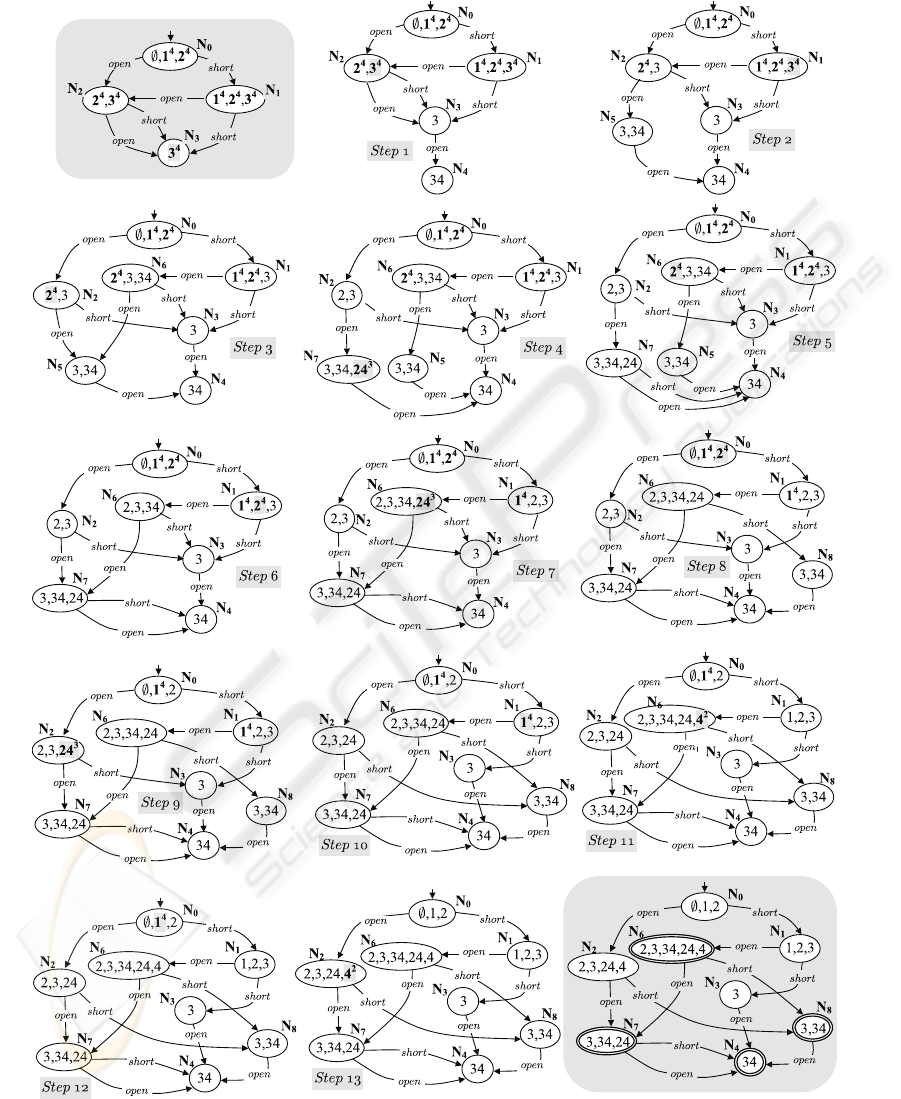
Figure 8: Tracing of the incremental computation of Isp(O

[4]

INCREMENTAL PROCESSING OF TEMPORAL OBSERVATIONS IN SUPERVISION AND DIAGNOSIS OF

DISCRETE-EVENT SYSTEMS

scenario (i): transition N

short

−−−→ N

is redirected

toward N

.For = open, scenario (j): no opera-

tion.

(11) B =(N

, {ω

},ω

), λ = {open}, P



= {ω

scenario (h): node N

is extended with P



and bud

, {ω

},ω

) is created.

(12) B =(N

, {ω

},ω

), λ = {open,ε}, P



{ω

,ω

}.For = open, scenario (j): no opera-

tion. For  = ε, scenario (b): no operation.

(13) B =(N

, {ω

},ω

), λ = {open}, P



= {ω

scenario (h): node N

is extended with index P



and a new bud (N

, {ω

},ω

) is created.

(14) B =(N

, {ω

},ω

), λ = {open,ε}, P



{ω

,ω

}.For = open, scenario (j): no opera-

tion. For  = ε, scenario (b): no operation.

Since the bud set B is empty, the core section ends.

The termination section (Line 113) qualiﬁes the ﬁnal

states of Isp(O

[4]

), namely N

, N

, and N

.As

expected, the last (shaded) graph in Fig. 8 represents

the same automaton Isp(O) in Fig. 4.

6 DISCUSSION

The technique for incremental construction of the in-

dex space is conceived in the context of dynamic

model-based diagnosis of DESs. In this realm, the

evolution of a system is monitored based on its model

and the observation it generates during operation. The

diagnostic engine is expected to react to each new

fragment of observation by generating a correspond-

ing set of candidate diagnoses based on the previous

behavior of the system and the new fragment. As

such, the diagnostic process is incremental in nature.

Model-based diagnosis of DESs is grounded on

two essential elements: the observation O and the

model M of the system. Roughly, the diagnostic en-

gine aims to explain O based on M. In so doing, a

subset of the behavior space of the system is deter-

mined and represented by a ﬁnite automaton, where

each path from the root to a ﬁnal state is a candidate

history of the system. Even if the automaton is ﬁnite,

the number of candidate histories may be unbounded

because of possible cycles within the automaton.

Each history is a sequence of component transi-

tions, where each transition can be either normal or

faulty. Consequently, each history corresponds to a

candidate diagnosis, namely the set of faulty transi-

tions within the history. Despite the unboundedness

of candidate histories, the number of possible diag-

noses is ﬁnite, since the total number of faulty transi-

tions of components in the system is ﬁnite too. Pre-

cisely, if F is the domain of faulty transitions, the

domain of candidate diagnoses is the powerset 2

including the empty diagnosis ∅ denoting a normal

(rather than faulty) behavior. However, due to the

constraints imposed by M and O, the set of candidate

diagnoses is in general a small subset of 2

, possibly

a singleton.

Considering a diagnostic problem ℘(O, M), where

O = ϕ

,...,ϕ

 is a temporal observation, we de-

ﬁne the static solution of the problem, ∆(℘(O, M)),

the set of candidate diagnoses relevant to the histo-

ries drawn from O based on M. Since we are in-

terested in updating the set of candidate diagnoses at

each new fragment of observation, we have to con-

sider the sequence of static solutions relevant to each

sub-problem ℘(O

[i]

, M), i ∈ [0 .. n], where O

[i]

is the

sub-observation ϕ

,...,ϕ

 up to the i-th fragment.

Note that, when i =0,wehaveanempty observation.

In other words, the diagnostic engine is expected

to generate a new static solution at the occurrence of

each newly-generated fragment of observation. This

is called the dynamic solution of ℘(O, M), namely

∆ = ∆(℘(O

[0]

, M)),...,∆(℘(O

[n]

, M)).

Another strong requirement for the diagnostic process

is that the model M of the system Σ is given only

intensionally, that is, in terms of the topology of Σ

(components and links among them) and the relevant

component models (communicating ﬁnite automata),

rather than extensionally, that is, in terms of the (pos-

sibly huge) automaton describing explicitly the sys-

tem behavior.

On the other hand, just as the observation graph

is not suitable for the diagnostic engine as is, and a

surrogate of it (the index space) is used instead, the

compositional model M turns to be inadequate as is,

and a surrogate of it is considered, namely the model

space of M, denoted Msp(M). Thus, for compu-

tational reasons, the diagnostic problem ℘(O, M) is

transformed by the diagnostic engine into a surro-

gate ℘(Isp(O), Msp(M)). As for the index space,

the model space is made up incrementally, following

a lazy evaluation approach: the model space is ex-

tended only when necessary for the diagnostic engine.

Essentially, a model space is a graph where nodes

correspond to possible system states, while edges are

marked by visible labels. Intuitively, a transition be-

tween nodes of the model space, N



−→ N



, occurs

when the new observation fragment involves label .

Both nodes and edges of the model space carry com-

piled diagnostic information: the dynamic solution

of the diagnostic problem can be generated based on

such information provided the index space is some-

how linked to the model space.

Speciﬁcally, each node  of Isp(O) must be deco-

rated with the set of model-space states which comply

Roughly, according to lazy evaluation, the generation

of node N



is triggered by the occurrence of label .

ICEIS 2006 - ARTIFICIAL INTELLIGENCE AND DECISION SUPPORT SYSTEMS

Figure 9: Experimental results: index-space computation-

time (y-axis) vs. number of observation fragments (x-axis).

with all the paths up to  in Isp(O). Such a decora-

tion is grounded on the common alphabet of the reg-

ular language of Isp(O) and of Msp(M), namely the

domain of visible labels. For example, if 

,...,



is a string of the language of Isp(O) ending at node

, and the same sequence of labels is also a string

of the language of Msp(M) ending at node N , then

the decoration of  will include N. Since several dif-

ferent strings may end at , the decoration of  will

include several nodes of Msp(M). Accordingly, the

Increment algorithm has been extended to cope with

decorated index spaces too.

7 CONCLUSION

Both the observation graph and the index space are

modeling primitives for representing temporal obser-

vations. Whereas the observation graph is the front-

end representation, suitable for modeling an observa-

tion while it is being received over a time interval, the

index space is a back-end representation, suitable for

model-based problem-solving and as a standard inter-

change format of uncertain observations among dis-

tinct application contexts. This paper has presented a

technique for constructing the index space incremen-

tally, while receiving observation fragments one at a

time. This is signiﬁcant whenever a nonmonotonic

processing step has to be performed after each ob-

servation fragment is received, as is when the tasks

of supervision and dynamic diagnosis (and state es-

timation, in general), are considered. The Increment

algorithm is an attempt to achieve the stated goals.

Experimental results, shown in Fig. 9, indicate that

the algorithm (implemented in C language) is sound,

complete, and efﬁcient. The diagram shows the time

(in seconds) to compute the index space of an obser-

vation composed of (up to) 600 fragments. The curve

on the top is relevant to the computation of each index

space from scratch. The curve on the bottom corre-

sponds to the incremental computation. The research

still needs to perform computational analysis, and to

gather further experimental results based on observa-

tions with different sizes and uncertainty degrees.

REFERENCES

Aho, A., Sethi, R., and Ullman, J. (1986). Compilers –

Principles, Techniques, and Tools. Addison-Wesley,

Reading, MA.

Baroni, P., Canzi, U., and Guida, G. (1997). Fault diag-

nosis through history reconstruction: an application

to power transmission networks. Expert Systems with

Applications, 12(1):37–52.

Baroni, P., Lamperti, G., Pogliano, P., and Zanella, M.

(1999). Diagnosis of large active systems. Artiﬁcial

Intelligence, 110(1):135–183.

Brusoni, V., Console, L., Terenziani, P., and Dupr

e, D. T.

(1998). A spectrum of deﬁnitions for temporal model-

based diagnosis. Artiﬁcial Intelligence, 102(1):39–80.

ob, D. and Wotawa, F. (2004). Introducing alias infor-

mation into model-based debugging. In Fifteenth In-

ternational Workshop on Principles of Diagnosis –

DX’04, pages 93–98, Carcassonne, F.

Lamperti, G. and Zanella, M. (2000). Uncertain tempo-

ral observations in diagnosis. In Fourteenth European

Conference on Artiﬁcial Intelligence – ECAI’2000,

pages 151–155, Berlin, D.

Lamperti, G. and Zanella, M. (2002). Diagnosis of discrete-

event systems from uncertain temporal observations.

Artiﬁcial Intelligence, 137(1–2):91–163.

Lamperti, G. and Zanella, M. (2003). Diagnosis of Active

Systems – Principles and Techniques, volume 741 of

The Kluwer International Series in Engineering and

Computer Science. Kluwer Academic Publisher, Dor-

drecht, NL.

Lamperti, G. and Zanella, M. (2004a). A bridged diagnostic

method for the monitoring of polymorphic discrete-

event systems. IEEE Transactions on Systems, Man,

and Cybernetics – Part B: Cybernetics, 34(5):2222–

2244.

Lamperti, G. and Zanella, M. (2004b). Dynamic diagno-

sis of active systems with fragmented observations.

In Sixth International Conference on Enterprise Infor-

mation Systems – ICEIS’2004, pages 249–261, Porto,

Mozeti

c, I. (1991). Hierarchical model-based diagno-

sis. International Journal of Man-Machine Studies,

35(3):329–362.

Roz

e, L. (1997). Supervision of telecommunication net-

work: a diagnoser approach. In Eighth International

Workshop on Principles of Diagnosis – DX’97, pages

103–111, Mont St. Michel, F.

Wotawa, F. (202). On the relationship between model-based

debugging and program slicing. Artiﬁcial Intelligence,

135(1–2):125–143.

INCREMENTAL PROCESSING OF TEMPORAL OBSERVATIONS IN SUPERVISION AND DIAGNOSIS OF

DISCRETE-EVENT SYSTEMS