Learning in Dynamic Environments:

Decision Trees for Data Streams

Jo˜ao Gama

1,2

and Pedro Medas

LIACC - University of Porto

Rua Campo Alegre 823, 4150 Porto, Portugal

Fac. Economics, University of Porto

Abstract. This paper presents an adaptive learning system for induction of for-

est of trees from data streams able to detect Concept Drift. We have extended

our previous work on Ultra Fast Forest Trees (UFFT) with the ability to detect

concept drift in the distribution of the examples. The Ultra Fast Forest of Trees

is an incremental algorithm, that works online, processing each example in con-

stant time, and performing a single scan over the training examples. Our system

has been designed for continuous data. It uses analytical techniques to choose the

splitting criteria, and the information gain to estimate the merit of each possible

splitting-test. The number of examples required to evaluate the splitting criteria

is sound, based on the Hoeffding bound. For multi-class problems the algorithm

builds a binary tree for each possible pair of classes, leading to a forest of trees.

During the training phase the algorithm maintains a short term memory. Given

a data stream, a ﬁxed number of the most recent examples are maintained in a

data-structure that supports constant time insertion and deletion. When a test is

installed, a leaf is transformed into a decision node with two descendant leaves.

The sufﬁcient statistics of these leaves are initialized with the examples in the

short term memory that will fall at these leaves. To detect concept drift, we main-

tain, at each inner node, a naive-Bayes classiﬁer trained with the examples that

traverse the node. While the distribution of the examples is stationary, the online

error of naive-Bayes will decrease. When the distribution changes, the naive-

Bayes online error will increase. In that case the test installed at this node is not

appropriate for the actual distribution of the examples. When this occurs all the

subtree rooted at this node will be pruned. This methodology was tested with two

artiﬁcial data sets and one real world data set. The experimental results show a

good performance at the change of concept detection and also with learning the

new concept.

Keywords: Concept Drift, Forest of Trees, Data Streams.

1 Introduction

Decision trees, due to its characteristics, are one of the most used techniques for data-

mining. Decision tree models are non-parametric, distribution-free, and robust to the

presence of outliers and irrelevant attributes. Tree models have high degree of inter-

pretability. Global and complex decisions can be approximated by a series of simpler

Gama J. and Medas P. (2004).

Learning in Dynamic Environments: Decision Trees for Data Streams.

In Proceedings of the 4th International Workshop on Pattern Recognition in Information Systems, pages 149-158

DOI: 10.5220/0002673001490158

 SciTePress

and local decisions. Univariate trees are invariant under all (strictly) monotone trans-

formations of the individual input variables. Usual algorithms that construct decision

trees from data use a divide and conquer strategy. A complex problem is divided into

simpler problems and recursively the same strategy is applied to the sub-problems. The

solutions of sub-problems are combined in the form of a tree to yield the solution of

the complex problem. Formally a decision tree is a direct acyclic graph in which each

node is either a decision node with two or more successors or a leaf node.Adecision

node has some condition based on attribute values. A leaf node is labelled with a con-

stant that minimizes a given loss function. In the classiﬁcation setting, the constant that

minimizes the 0-1 loss function is the mode of the classes that reach this leaf.

Data streams are, by deﬁnition, problems where the training examples used to con-

struct decision models come over time, usually one at time. In usual real-world applica-

tions the data ﬂows continuously at high-speed. In these situations is highly unprovable

the assumption that the examples are generated at random according to a stationary

probability distribution. At least in complex systems and for large time periods, we

should expect changes in the distribution of the examples. A natural approach for this

incremental tasks are adaptive learning algorithms, that is incremental learning algo-

rithms that take into account concept drift. In this paper we present UFFT, an algorithm

that generates forest-of-trees for data streams. The main contributions of this work are

a fast method, based on discriminant analysis, to choose the cut point for splitting tests,

the use of a short-term memory to initialize new leaves, the use of functional leaves to

classify test cases, and the ability to detect concept drift.

The paper is organized as follows. In the next section we present related work in the

area of incremental decision-tree induction. In Section 3, we present the main issues of

our algorithm. The system has been implemented, and evaluated in a set of benchmark

problems. The preliminary results are presented in Section 4. In the last section we

resume the main contributions of this paper, and point out some future work.

2 Related Work

In this section we analyze related work in two dimensions. One dimension is related

to methods to deal with concept drift. The other dimension is related to the induction

of decision trees from data streams. Other works related to the work presented here

include the use of more power classiﬁcation strategies at tree leaves, and the use of

forest of trees.

In the literature of machine learning, several methods have been presented to deal

with time changing concepts [13,18,11,12,7]. The two basic methods are based on

Temporal Windows where the window ﬁxes the training set for the learning algorithm

and Weighting Examples that ages the examples, shrinking the importance of the oldest

examples. These basic methods can be combined and used together. Both weighting and

time window forgetting systems are used for incremental learning. A method to choose

dynamically the set of old examples that will be used to learn the new concept faces

several difﬁculties. It has to select enough examples to the learner algorithm and also

to keep old data from disturbing the learning process. Older data will have a different

probability distribution from the new concept. A larger set of examples allows a better

150

generalization if no concept drift happened since the examples arrived [18]. The sys-

tems using weighting examples use partial memory to select the more recent examples,

and therefore probably within the new context. Repeated examples are assigned more

weight. The older examples, according to some threshold, are forgotten and only the

newer ones are used to learn the new concept model [12].

Learning algorithms can learn a new concept using all the previouslyseen examples,

thus not forgetting old examples, full memory, or use a data management system to

locate the time point t when the new concept started, time window.

When a drift concept occurs the older examples become irrelevant. We can apply a

time window on the training examples to learn the new concept description only from

the most recent examples. The time window can be improved by adapting its size. [18]

and [11] present several methods to choose a time window dynamically adjusting the

size using heuristics to track the learning process. The methods select the time win-

dow to include only examples on the current target concept. [12] presents a method to

automatically select the time window size in order to minimize the generalization error.

The CVFDT [7] is an algorithmfor mining decisiontrees from continuous-changing

data streams. It extends the VFDT [3] system with the ability to detect changes in the

underlying distribution of the examples. At each node CVFDT maintains the sufﬁcient

statistics to compute the splitting-test. Each time an example traverses the node the

statistics are updated. After seeing n

min

examples, the splitting-test is recomputed. If

a new test is chosen, the CVFDT starts growing an alternate subtree. The old one is re-

placed only when the new one becomes more accurate. This is a fundamental difference

to our method. The CVFDT uses old data to maintain two subtrees. The UFFT with drift

detection prunes the subtree when detecting a new context and only uses the current ex-

ample. The CVFDT constantly veriﬁes the validity of the splitting test. The UFFT only

veriﬁes that the examples at each node have a stationary distribution function.

Kubatand Widmer [13] describea system that adapts to drift in continuous domains.

[10] show the application of several methods of handling concept drift with an adaptive

time window on the training data, select representative training examples or weight the

training examples. Those systems automatically adjust the window size, the example

selection and the example weighting to minimize the estimated generalization error.

In the ﬁeld of combining classiﬁers several algorithms generate forest of trees. One

of the most used strategies is Bagging [1] where different trees are obtained by using

bootstrap samples from the training set. Breiman [2] presented an algorithm to ran-

domly generate a forest of trees. Each tree depends on the values of a random vector

sampled independentlyand with the same distribution for all trees in the forest. Breiman

shows that using a random selection of features to split each node yields error rates that

compare favorably to Adaboost. In our case there is no random factor. The forest of

trees is obtained by decomposing a k-class problem into k(k − 1)/2 binary problems.

3 Ultra-Fast Forest Trees - UFFT

The UFFT [5] is an algorithm for supervised classiﬁcation learning, that generates a

forest of binary trees. The algorithm is incremental, with constant time for processing

each example, works on-line, and uses the Hoeffding bound to decide when to install

151

a splitting test in a leaf leading to a decision node. UFFT is designed for continuous

data. It uses analytical techniques to choose the splitting criteria, and the information

gain to estimate the merit of each possible splitting-test. For multi-class problems, the

algorithm builds a binary tree for each possible pair of classes leading to a forest-of-

trees. During the training phase the algorithm maintains a short term memory. Given

a data stream, a limited number of the most recent examples are maintained in a data

structure that supports constant time insertion and deletion. When a test is installed,

a leaf is transformed into a decision node with two descendant leaves. The sufﬁcient

statistics of the leaf are initialized with the examples in the short term memory that

will fall at that leaf. The UFFT [5] has shown good results with several problems and

large and medium datasets. In this work we incorporate in UFFT system the ability to

support Concept Drift Detection. To detect concept drift, we maintain, at each inner

node, a naive-Bayes classiﬁer trained with the examples that traverse the node. While

the distribution of the examples is stable, the online error of naive-Bayes will decrease.

When the distribution function of the examples changes, the online error of the naive-

Bayes at the elad will increase. In that case we decide thatthe test installed at this node is

not appropriate for the actual distribution of the examples. When this occurs the subtree

rooted at this node will be pruned. The algorithm forget the sufﬁcient statistics and

learns the new concept with only the examples in the new concept. The drift detection

method will always check the stability of the distribution function of the examples at

each decision node. In the following sections we provide detailed information about the

most relevant aspects of the system.

The Splitting Criteria The UFFT starts with a single leaf. When a splitting test is in-

stalled at a leaf, the leaf becomes a decision node, and two descendant leaves are gen-

erated. The splitting test has two possible results each conducting to a different leave..

The value True is associated with one branch and the value False, whith the other. The

splitting tests are over a numerical attribute and are of the form attribute

≤ value

We use the analytical method for split point selection presented in [14]. We choose,

for all numerical attributes, the most promising value

. The only sufﬁcient statistics

required are the mean and variance per class of each numerical attribute. This is a ma-

jor advantage over other approaches, as the exhaustive method used in C4.5 [17] and

in VFDTc [8], because all the necessary statistics are computed on the ﬂy. This is a

desirable property on the treatment of huge data streams because it guarantees constant

time processing each example.

The analytical method uses a modiﬁedform of quadratic discriminant analysis to in-

clude different variances on the two classes

. This analysis assumes that the distribution

of the values of an attribute follows a normal distributionfor both classes. Let φ(¯x, σ)=

√

2π

exp



−

(x−¯x)

2σ



be the normal density function, where ¯x and σ

are the sample

mean and variance of the class. The class mean and variance for the normal density

function are estimated from the sample set of examples at the node. The quadratic dis-

criminant splits the X-axis into three intervals (−∞,d

), (d

, ∞) where d

and d

are the possible roots of the equation p(−)φ{(¯x

−

,σ

−

)} = p(+)φ{(¯x

,σ

)}

The reader should note that in UFFT any n-class problem is decomposed into n(n − 1)/2

two-class problems.

152

where p(−) denotes the estimated probability than an example belongs to class −.We

pretend a binary split, so we use the root closer to the sample means of both classes.

Let d be that root. The splitting test candidate for each numeric attribute i will be of

the form Att

≤ d

. To choose the best splitting test from the candidate list we use

an heuristic method. We use the information gain to choose, from all the splitting point

candidates, the best splitting test. To compute the informationgain we need to construct

a contingency table with the distribution per class of the number of examples lesser and

greater than d

Att

≤ d

Att

Class + p

Class − p

−

The information kept by the tree is not sufﬁcient to compute the exact number of ex-

amples for each entry in the contingency table. Doing that would require to maintain

information about all the examples at each leaf. With the assumption of normality, we

can compute the probability of observing a value less or greater than d

. From these

probabilities and the distribution of examples per class at the leaf we populate the con-

tingency table. The splitting test with the maximum information gain is chosen. This

method only requires that we maintain the mean and standard deviation for each class

per attribute. Both quantities are easily maintained incrementally. In [8] the authors

presented an extension to VFDT to deal with continuous attributes. They use a Btree to

store continuous attribute-values with complexity O(nlog(n)). The complexity of the

proposed method here is O(n). This is why we denote our algorithm as ultra-fast. Once

the merit of each splitting has been evaluated, we have to decide on the expansion of

the tree. This problem is discussed in the next section.

From Leaf to Decision Node To expand the tree, the a test attribute

≤ d

is installed

in a leaf, and the leaf becomes a decision node with two new descendant leaves. To

expand a leaf two conditions must be satisﬁed. The ﬁrst one requires the information

gain of the selected splitting test to be positive. That is, there is a gain in expanding

the leaf against not expanding. The second condition, it must exist statistical support in

favor of the best splitting test, is asserted using the Hoeffding bound as in VFDT [3].

The innovation in UFFT is the method used to determine how many examples

are needed to evaluate the splitting criteria. As we have pointed out, a new instance

does not automatically triggers the splitting decision criteria. Only after receiving n

min

examples since the last evaluation instances will the algorithm execute the splitting

test criteria. The number of examples needed till the next evaluation is computed as

(1.0/(2 ∗ δ)) ∗ log(2.0/), with conﬁdence 1 − δ and  easily derived from the Hoeffd-

ing bounds [16].

When new nodes are created, the short term memory is used. This is described in

the following section.

Short Term Memory When a new leaf is created its sufﬁcient statistics are initialized to

zero. The new leaves are trained with the past examples that are in the new concept. We

use a short term memory that maintains a limited number of the most recent examples.

This short term memory is used to update the statistics at the new leaves when they are

153

created. The examples in the short term memory traverse the tree. The ones that reach

the new leaves will update the sufﬁcient statistics of the tree. The data structure used

in our algorithm supports constant time insertion of elements at the beginning of the

sequence and constant time removal of elements at the end of the sequence.

Classiﬁcation strategies at leaves To classify an unlabelled example, the example tra-

verses the tree from the root to a leaf. It follows the path established, at each de-

cision node, by the splitting test at the appropriate attribute-value. The leaf reached

classiﬁes the example. The classiﬁcation method is a naive-Bayes classiﬁer. The use

of the naive-Bayes classiﬁers at the tree leaves does not enter any overhead in the

training phase. At each leaf we maintain sufﬁcient statistics to compute the informa-

tion gain. These are the necessary statistics to compute the conditional probabilities of

P (x

|Class) assuming that the attribute values follow, for each class, a normal dis-

tribution. Let l be the number of attributes, and φ(¯x, σ) denotes the standard normal

density function for the values of attribute i that belong to a given class. Assuming

that the attributes are independent given the class, the Bayes rule will classify an ex-

ample in the class that maximizes the a posteriori conditional probability, given by:

P (C

|x) ∝ log(Pr(C

)) +



k=1

log(φ(¯x

)). There is a simple motivation for this

option. UFFT only changes a leaf to a decision node when there is a sufﬁcient number

of examples to support the change. Usually hundreds or even thousands of examples

are required. To classify a test example, the majority class strategy only use the infor-

mation about class distributions and does not look for the attribute-values. It uses only a

small part of the available information, a crude approximation to the distribution of the

examples. On the other hand, naive-Bayes takes into account not only the prior distri-

bution of the classes, but also the conditional probabilities of the attribute-values given

the class. In this way, there is a much better exploitation of the information available at

each leaf.

Forest of Trees The splitting criteria only applies to two class problems. In the original

paper [14] and for a batch-learning scenario, this problem was solved using, at each

decision node, a 2-means cluster algorithm to group the classes into two super-classes.

Obviously, the cluster method can not be applied in the context of learning from data

streams. We propose another methodology based on round-robin classiﬁcation [4]. The

round-robin classiﬁcation technique decomposes a multi-class problem into k binary

problems, that is, each pair of classes deﬁnes a two-classes problem. In [4] the author

shows the advantages of this method to solve n-class problems. The UFFT algorithm

builds a binary tree for each possible pair of classes. For example, in a three class

problem (A,B, and C) the algorithm grows a forest of binary trees, one for each pair:

A-B, B-C, and A-C. In the general case of n classes, the algorithm grows a forest of

n(n−1)

binary trees. When a new example is received during the tree growing phase

each tree will receive the example if the class attached to it is one of the two classes in

the tree label. Each example is used to train several trees and neither tree will get all

examples. The short term memory is common to all trees in the forest. When a leaf in

a particular tree becomes a decision node, only the examples corresponding to this tree

are used to initialize the new leaves.

154

Fusion of Classiﬁers When doing classiﬁcation of a test example, the algorithm send

the example to all trees in the forest. The example will traverse the tree from root to

leaf and the classiﬁcation registered. Each of the trees in the forest makes a prediction.

This prediction takes the form of a probability class distribution. Taking into account

the classes that each tree discriminates, these probabilities are aggregated using the sum

rule [9]. The most probable class is used to classify the example. Note that some exam-

ples will be forced to be classiﬁed erroneously by some of the binary base classiﬁers.

this is because each classiﬁer must label all examples as belonging to one of the two

classes it was trained on.

Concept Drift Detection The UFFT algorithm maintains, at each node of all decision

trees, a naive-Bayes classiﬁer. The naive-Bayesmodel is constructed usingthe examples

that traverse the node. The basic idea of the drift detection method is to control the

error-rate of the naive-Bayes classiﬁer. If the distribution of the examples that traverse

a node is stationary, the error rate of naive-Bayes decreases. If there is a change on the

distribution of the examples the naive-Bayes error will increase [15]. When the system

detect an increase of the naive-Bayes error in a given node, an indication of a change

in the distribution of the examples, this suggest that the splitting-test that have been

installed at this node is no more appropriate. In such cases, all the subtree rooted at that

node is pruned, and the node becomes a leaf. All the sufﬁcient statistics of the leaf are

initialized using the examples in the new context from the short term memory.

We designate as context a set of contiguous examples where the distribution is sta-

tionary. We assume that the data stream is a set of contexts. The goal of the method is

to detect when in the sequence of examples of the data stream there is a change from

one context to another context.

When a new example becomes available, it will cross the corresponding binary

decision trees from the root through a leaf. At each node, the naive Bayes installed at

that node classify the example. The example will be or correcty classiﬁed or an error

occur. For a set of examples the error is a random variable from Bernoulli trials. The

Binomial distribution gives the general form of the probability for the random variable

that represents the number of errors in a sample of n examples. We use the following

estimator for the true error of the classiﬁcation function p

≡ (error

/i) where i is the

number of examples and error

is the number of examples misclassiﬁed in the present

context.

A cause for estimation error is the variance of the estimate. Even with an unbiased

estimator, the observed value of the estimator is likely to vary from one experiment

to another. The variance of the distribution governing the estimator decreases as the

number of examples increase. We estimate the variance using the following estimator

to the standard deviation s

≡



∗(1−p

)

, where i is the number of examples observed

within the present context. For sufﬁcient large values of the example size, the Binomial

distribution is closely approximated by a Normal distribution with the same mean and

variance. Considering that the probability distribution is unchanged when the context is

static, then the N% conﬁdence interval for p with n>30 examples is approximately

p ± α ∗ s

. The drift detection method manages two registers during the training of

155

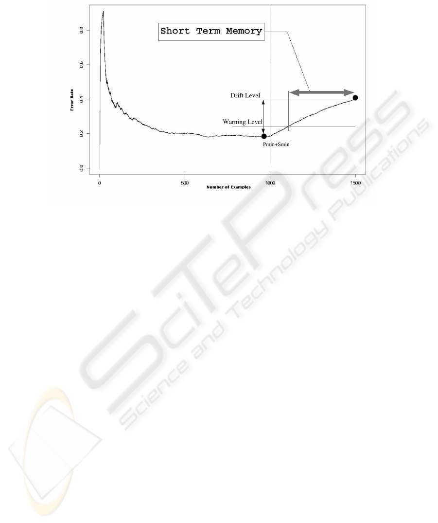
Fig.1. Dynamically constructed Time Window. The horizontal line marks the change of context.

the learning algorithm, p

min

and s

min

. Every time a new example i is processed those

values are updated when p

+ s

is lower or equal than p

min

+ s

min

We use a warning level to ensure the optimal size of the time window. The time

windows will contain the old examples that are on the new context. And a minimal

number of examples on the old context. This warning level is reached when a new

examples, i, is suspected of being in the new context, p

+ s

≥ p

min

+1.5∗ s

min

. This

example will be the start point of the time window. The time window is closed when

the current p

+ s

is greater or equal than p

min

+3∗ s

min

. This will be where the

new context is declared.Figure1 details the time window structure. With this method of

learning and forgetting we ensure a way to continuously keep a model better adapted to

the present context. The method uses the information already available to the learning

algorithm and does not require additional computational resources.

4 Experimental Work

The experimental work was done using artiﬁcial data previously used in [13] and a real

time problem described in [6]. All datasets are available in the Internet.

Artiﬁcial Datasets The artiﬁcial problems allow us to choose the point of drift and

the form of changing drift. One dataset (circles) has a gradual context drift. The other

(sine2) has an abrupt context drift. Both datasets have 2 contexts. 10000 examples in

each context. Each dataset is composed of 20000 random generated examples. The test

datasets have 100 examples from the last context in the train dataset. This characteris-

tics allow us to assess the performanceof the method in various conditions. The dataset

156

Artiﬁcial Detect Drift

Dataset Yes No

Abrupt Drift 0.00 0.02

Gradual Drift 0.01 0.1

Lower Upper Bound UFFT

Test Set Bound All Data Last Year Drift Detection

Last Day 0.08 0.187 0.125 0.08

Last Week 0.15 0.235 0.247 0.16

Fig.2. Error rates on Drift Detection. Artiﬁcial Data (left) and Electricity Data (wright).

with an abrupt concept drift has two relevant attributes. The results (ﬁgure 2) show a

signiﬁcantly advantage for using UFFT with context drift detection versus UFFT with

no drift detection. For both datasets. The results obtained for the UFFT with drift de-

tection shown no overhead on the processing time and no need of more computational

resources.

The Electricity Market Dataset The data used in this experiments was ﬁrst described

by M. Harries [6]. The data was collected from the Australian New South Wales Elec-

tricity Market. The prices are not ﬁxed and are affected by demand and supply of the

market. The prices in this market are set every ﬁve minutes. We performed a several ex-

periments for detecting the lower and upper bound of the error rate. The results appear

in ﬁgure 2. To evaluate the drift detection method suggested we designed three sets of

experiments. The sets of experiments were conducted to ﬁnd a lower and upper bound

to the performance of the proposed method. We used two different test datasets. One

test dataset with only the examples referring to the last day observed and the other with

the last week of examples recorded. All the other examples are in the train dataset. The

experiment using UFFT with drift detection show a signiﬁcant better result than those

obtained for the lower bounds. This is a real world dataset where we do not know where

the context is changing.

5 Conclusions

This work presents an incremental learning algorithm appropriate for processing high-

speed numerical data streams with the capability to adapt to concept drift. The UFFT

system can process new examples as they arrive, using a single scan of the training data.

The method is fast, based on discriminant analysis, to choose the cut point for splitting

tests. The sufﬁcient statistics required by the analytical method can be computed in an

incremental way, guaranteeing constant time to process each example. This analytical

method is restricted to two-class problems. We use a forest of binary trees to solve

problems with more than 2 classes. Other contributions of this work are the use of

a short-term memory to initialize new leaves, the use of functional leaves to classify

test cases, and the use of a dynamic and sound method to decide how many examples

are needed to evaluate candidate splits. The empirical evaluation of our algorithm, clear

shows the advantages of using more powerfulclassiﬁcation strategies at tree leaves. The

performance of UFFT when using naive-Bayes classiﬁers at tree leaves is competitive

to the state of the art in batch decision tree learning, using much less computational

resources. The main contribution of this work is the ability to detect changes in the

class-distribution of the examples. The system maintains, at each inner node, a naive-

Bayes classiﬁer trained with the examples that cross the node. While the distribution

157

of the examples is stationary, the online error of naive-Bayes will decrease. When the

distribution changes, the naive-Bayes online error will increase. In that case the test

installed at this nodeis not appropriate for the actual distribution of the examples.When

this occurs all the subtree rooted at this node will be pruned. naive-Bayes classiﬁer

central idea on this work is the control of the training dataset that goes through to the

learning algorithm. The algorithm forget the old examples and learns the new concept

with only the examples in the new concept. This methodology was tested with two

artiﬁcial data sets and one real world data set. The experimental results show a good

performance at the change of concept detection and also with learning the new concept.

Acknowledgments: The authors reveal its gratitude to the ﬁnancial support given by the FEDER,

and the Plurianual support attributed to LIACC. This work was developed in the context of the

project ALES (POSI/SRI/39770/2001).

References

1. L. Breiman. Bagging predictors. Machine Learning, 24, 1996.

2. Leo Breiman. Random forests. Technical report, University of Berkeley, 2002.

3. P. Domingos and G. Hulten. Mining high-speed data streams. In Knowledge Discovery and

Data Mining, pages 71–80, 2000.

4. J. F¨urnkranz. Round robin classiﬁcation. Journal of Machine Learning Research, 2:721–747,

2002.

5. J. Gama, P. Medas, and R. Rocha. Forest trees for on-line data. In ACM Symposium on

Applied Computing - SAC04, 2004.

6. Michael Harries. Splice-2 comparative evaluation: Electricity pricing. Technical report, The

University of South Wales, 1999.

7. Geoff Hulten, Laurie Spencer, and Pedro Domingos. Mining time-changing data streams. In

Knowledge Discovery and Data Mining, 2001.

8. J.Gama, R. Rocha, and P.Medas. Accurate decision trees for mining high-speed data streams.

In Procs. of the 9th ACM SigKDD Int. Conference in Knowledge Discovery and Data Mining.

ACM Press, 2003.

9. J. Kittler. Combining classiﬁers: A theoretical framework. Pattern analysis and Applications,

Vol. 1, No. 1, 1998.

10. R. Klinkenberg. Learning drifting concepts: Example selection vs. example weighting. In-

telligent Data Analysis, 2004.

11. R. Klinkenberg and I. Renz. Adaptive information ﬁltering: Learning in the presence of

concept drifts. In Learning for Text Categorization, pages 33–40. AAAI Press., 1998.

12. Ralf Klinkenberg and Thorsten Joachims. Detecting concept drift with support vector ma-

chines. In Pat Langley, editor, Proceedings of ICML-00, 17th International Conference on

Machine Learning, pages 487–494, Stanford, US, 2000. Morgan Kaufmann Publishers, San

Francisco, US.

13. M. Kubat and G. Widmer. Adapting to drift in continuous domain. In Proceedings of the 8th

European Conference on Machine Learning, pages 307–310. Spinger, 1995.

14. W.-Y. Loh and Y.-S. Shih. Split selection methods for classiﬁcation trees. Statistica Sinica,

1997.

15. Tom Mitchell. Machine Learning. McGraw Hill, 1997.

16. R. Motwani and P. Raghavan. Randomized Algorithms. Cambridge University Press, 1997.

17. R. Quinlan. C4.5: Programs for Machine Learning. Morgan Kaufmann Publishers, Inc.,

1993.

18. Gerhard Widmer and Miroslav Kubat. Learning in the presence of concept drift and hidden

contexts. Machine Learning, 23:69–101, 1996.

158